Code
monthly_income                   <- 4995
monthly_social_security_benefits <- 1710
monthly_cost_of_living <- 3500Juliet just turned 20 and is ready to start her adult life. She’s landed a stable, well-paid job and her new journey begins. This time, life unfolds without Romeo. Think she can’t handle it? You might be surprised.
Juliet feels anxious about her future. Each month she have to choose how to balance spending, saving, and investing for what’s ahead. She’s keen to avoid poor decisions. Juliet seeks clear, rational advice tailored to her needs—not the generic advice that’s all over the internet. She aims to make informed, personalized financial choices that align with her present knowledge and future plans. She needs a clear set of recommendations to know how much to save and how to invest 1.
Let’s follow Juliet’s example to craft a straightforward financial report for a single-person household. We will be using our new R4GoodPersonalFinances R package that implements (with our modifications) the theoretical model invented and described in Lifetime Financial Advice: A Personalized Optimal Multilevel Approach by Thomas M. Idzorek and Paul D. Kaplan (Idzorek and Kaplan 2024).
We aim to explore scenarios that an individual might encounter, based on realistic assumptions about market returns and living expenses in a big Polish city. These scenarios reflect a consistent, median-level income. We focus on income and spending estimates for Poland, using Polish złoty (PLN). However, you can adapt these scenarios to any currency or country-specific factors.
monthly_income <- 4995
monthly_social_security_benefits <- 1710
monthly_cost_of_living <- 3500Juliet, a 20-year-old young woman that leaves in a big city in Poland, chooses to stay single. She imagines this will be her lifelong path.
Juliet has just got a job, so she expects a steady income of 4’995 PLN net salary per month (real / inflation-adjusted). When she retires (at the age of 60 or later) she will receive a pension from Polish social security (emerytura ZUS) of 1’710 PLN per month (in today’s money and inflation-adjusted).
Juliet plans to spend 3’500 PLN each month on her basic needs. This covers her essential, non-discretionary expenses. Beyond that, she would like to allocate some funds for discretionary spending – the things that bring her joy.
Juliet holds modest savings of 1’500 PLN, already invested in two assets: a global stock ETF and Polish inflation-protected bonds, known as EDO.
Juliet aims to apply a lifecycle model to pinpoint her optimal discretionary spending and asset allocation. She also wants to explore how her discretionary spending might shift if she retires at various ages.
Welcome to R4GoodPersonalFinances version 1.1.0!Cite the package: citation('R4GoodPersonalFinances')Package documentation: https://r4goodacademy.github.io/R4GoodPersonalFinances/To learn more, visit: https://www.r4good.academy/... and Make Optimal Financial Decisions!We start with setting one common current_date for all analyses in the report. Let’s assume that the current date is 2025-01-01. We could set the current_date parameter in each function call, but we can also set it as a global option for the entire R session - like in our example.
If we didn’t set the current_date parameter, it would be set to the current computer date by default. As a result, the report cold not be the same if rendered for different dates. So for reproducibility, we set the current_date to this arbitrary date 2025-01-01 for the whole R session.
options("R4GPF.current_date" = "2025-01-01")First, we need to create an object of HouseholdMember class that represents Juliet.
juliet <- HouseholdMember$new(
  name       = "Juliet",
  birth_date = "2005-01-01"
)
juliet
── "Juliet" ℹ Birth date: 2005-01-01ℹ Current age: 20 yearsℹ Max age: 100 yearsℹ Max lifespan: 80 yearsℹ Gompertz mode: NAℹ Gompertz dispersion: NAℹ Life expectancy: NA yearsJuliet came into this world on January 1, 2005—exactly 20 years before the report’s date, January 1, 2025. By default, her maximum age is 100 years. So, her remaining lifespan is 80 years, calculated as maximum age minus current age (100 - 20 = 80).
We haven’t determined mode and dispersion for the Gompertz model yet, so life expectancy remains unclear. Let’s address that now.
Let’s find Julia’s Gompertz parameters: mode and dispersion. We’ll calculate these using data from a typical 20-year-old Polish woman and then apply them to Julia.
Discover why Gompertz parameters matter and how to model them here: How to model our probability of survival?
gompertz_parameters <-
  get_default_gompertz_parameters(
    age     = juliet$calc_age(),
    country = "Poland",
    sex     = "female"
  )

juliet$mode       <- gompertz_parameters$mode
juliet$dispersion <- gompertz_parameters$dispersion
juliet$max_age    <- gompertz_parameters$max_age
juliet
── "Juliet" ℹ Birth date: 2005-01-01ℹ Current age: 20 yearsℹ Max age: 97.8 yearsℹ Max lifespan: 77.8 yearsℹ Gompertz mode: 89ℹ Gompertz dispersion: 10.08ℹ Life expectancy: 83.3 yearsWe estimate Juliet could live up to 97.8 years, with an expected lifespan of about 83.3 years.
Let’s start a household with Juliet. Juliet is the lone member, but she is welcome to add others as needed in the future.
household <- Household$new()
household$add_member(juliet)
household
── Household ───────────────────────────────────────────────────────────────────ℹ Current date: 2025-01-01ℹ Household lifespan: 78 yearsℹ Consumption impatience preference: 0.04ℹ Smooth consumption preference: 1ℹ Risk tolerance: 0.5── Household members ──── "Juliet" ℹ Birth date: 2005-01-01ℹ Current age: 20 yearsℹ Max age: 97.8 yearsℹ Max lifespan: 77.8 yearsℹ Gompertz mode: 89ℹ Gompertz dispersion: 10.08ℹ Life expectancy: 83.3 yearsYou can see that we successfully added Juliet to her household.
Juliet’s household comes with preset preferences. Key ones include:
Future posts will explore these preferences in detail and offer tips on customization. For now, let’s assume that default values of those preferences are sensible and will work for Juliet well enough.
Juliet’s lifespan matches that of her household since she’s its sole member. You can visualize the lifespans of household members by plotting their age-of-death probability distributions and life expectancy.
household |> plot_life_expectancy()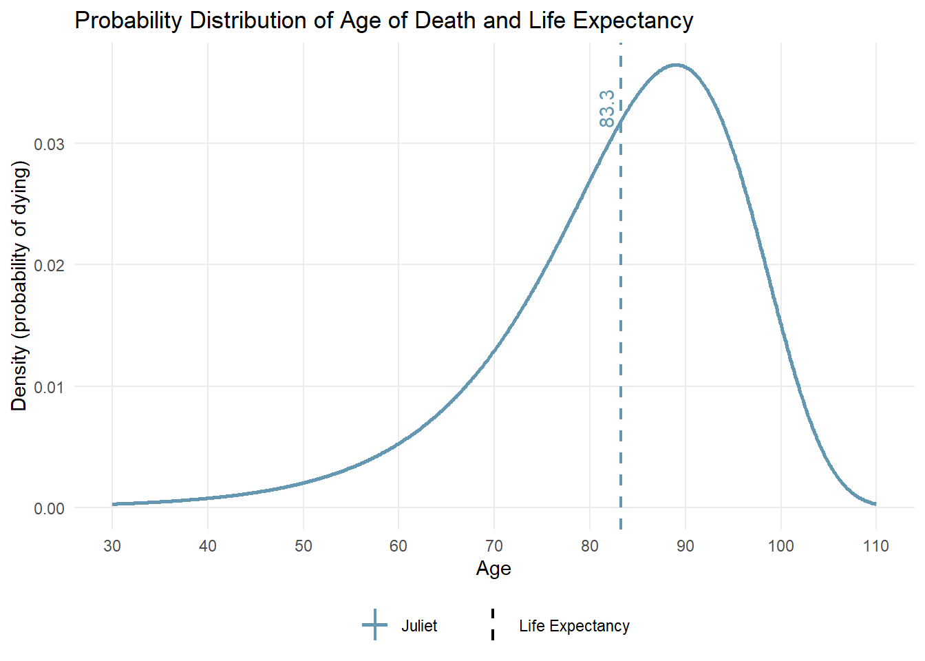
On the plot, Juliet sees her life expectancy is 83.3 years. She knows this is just an estimate; her actual lifespan could be shorter or longer. The life-cycle model takes into account all probabilities tied to different lifespans.
She may consider in the future adjusting the Gompertz parameters to match her life expectancy expectations. For now, she’s content with the defaults.
We need to define both income and spending in “real” terms to account for inflation over time. For instance, setting a real income of 1 000 PLN implies it maintains its purchasing power and increases with inflation. This way, years later, you can still buy what 1 000 PLN can buy today. This is a reasonable, though optimistic, expectation for salary and more realistic for inflation-adjusted social security pensions.
We need to set expected annual income and expenses. If you have a monthly amount, multiply it by 12 for the yearly total.
We’ll demonstrate next how to define cash flow streams linked to events affecting a household member. In this case, we’ll focus on income changes tied to a retirement event and Juliet’s age.
retirement eventretirement_start_age <- 60As Juliet expects to retire at the age of 60 years, we set the retirement event to start at this age. We also assume that Juliet will be retired till the end of her life.
juliet$set_event("retirement", start_age = retirement_start_age)Juliet expects that in her lifetime she will be receiving two income streams: salary income and social security pension income.
The income needs to be defined as net disposable income - the after-tax income that Juliet can spend on stuff she needs and wants (non-discretionary and discretionary spending).
Juliet is moderately optimistic about her future income. She expects to make 4’995 PLN net salary per month (after taxes). This is coincidentally the median net salary in Poland in November 20242.
Juliet also expects to receive a pension from Polish social security (emerytura ZUS) of 1’710 PLN per month. This is coincidentally the net minimum social security pension in Poland in 20253.
Juliet is rather conservative in this believe, as her social security benefits will be probably higher than the minimum, especially if she decides to work longer, and claims the benefits at a later age (more about this later).
Alright, we have what we need to set up rules triggering different income streams for Juliet, based on her age and the retirement event.
We’re defining a salary income stream, which provides funds while Juliet isn’t retired. The social security benefits stream activates when Juliet retires at 60 (Poland’s minimum age for women to claim these benefits) or later.
household$expected_income <-
  list(
    "salary income" = c(
      glue::glue(
        "is_not_on('Juliet', 'retirement') ~ {monthly_income * 12}"
        )
    ),
    "social security benefits" = c(glue::glue(
      "is_on('Juliet', 'retirement') & age('Juliet') >= 60 ~ ",
      "{monthly_social_security_benefits * 12}"
    ))
  )
household$expected_income
$`salary income`
[1] "is_not_on('Juliet', 'retirement') ~ 59940"
$`social security benefits`
[1] "is_on('Juliet', 'retirement') & age('Juliet') >= 60 ~ 20520"Juliet must identify her essential expenses. Non-discretionary spending covers basic needs such as food, clothing, housing, transport, and medical care. She estimates these costs at 3,500 PLN monthly for living alone in a big city in Poland 4.
Let’s keep it simple. Non-discretionary spending stays the same, even after retirement. But discretionary spending? That changes. Juliet wants to know how much is optimal for her.
$`total non-discretionary spending`
TRUE ~ 42000Non-discretionary spending can vary even within the same category. Take transport, for instance. City bus fares might be essential, yet driving a personal car could be viewed as optional. The distinction often hinges on individual circumstances and assessments.
Let’s set up Juliet’s portfolio with a simple template, mostly keeping the defaults. Juliet invests her savings in two assets: a global stock index fund or ETF, and Polish inflation-protected bonds (EDO).
She already has some savings in Polish inflation-protected bonds: 1’000 PLN in a taxable account and 500 PLN in a tax-advantaged account such as IKE.
Juliet views her human capital (discounted future income) and liabilities (discounted future non-discretionary spending) as bond-like—steady and rather uncorrelated to the stock market. This perspective makes sense for many but should be tailored to fit each person’s situation5.
We’ll build Juliet’s portfolio, incorporating relevant defaults for Poland, such as tax rates. We’ll also calculate effective tax rates and the optimal asset allocation for her portfolio.
portfolio <- create_portfolio_template()

portfolio$accounts$taxable       <- c(0, 1000)
portfolio$accounts$taxadvantaged <- c(0, 500)

portfolio$weights$liabilities[1] <- 0.10
portfolio$weights$liabilities[2] <-  1 - portfolio$weights$liabilities[1]

portfolio$weights$human_capital[1] <- 0.10
portfolio$weights$human_capital[2] <-  1 - portfolio$weights$human_capital[1]

portfolio <-
  portfolio |>
  calc_effective_tax_rate(
    tax_rate_ltcg            = 0.19,
    tax_rate_ordinary_income = 0.19
  )

portfolio <-
  calc_optimal_asset_allocation(
    household    = household,
    portfolio    = portfolio
  )
We can now display portfolio assumptions and calculation results in the R console.
portfolio── Portfolio ───────────────────────────────────────────────────────────────────── Market assumptions ──── Expected real returns: # A tibble: 2 × 3
name expected_return standard_deviation
<chr> <dbl> <dbl>
1 GlobalStocksIndexFund 0.0461 0.15
2 InflationProtectedBonds 0.02 0 ── Correlation matrix: GlobalStocksIndexFund InflationProtectedBonds
GlobalStocksIndexFund 1 0
InflationProtectedBonds 0 1── Weights ── human_capital liabilities
GlobalStocksIndexFund 0.1 0.1
InflationProtectedBonds 0.9 0.9── Accounts ──# A tibble: 3 × 4
name taxable taxadvantaged total
<chr> <dbl> <dbl> <dbl>
1 GlobalStocksIndexFund 0 0 0
2 InflationProtectedBonds 1000 500 1500
3 total 1000 500 1500── Pre-tax ──# A tibble: 2 × 7
name turnover income_qualified capital_gains_long_term
<chr> <dbl> <dbl> <dbl>
1 GlobalStocksIndexFund 0.04 0 1
2 InflationProtectedBonds 0.04 0 1
income capital_gains cost_basis
<dbl> <dbl> <dbl>
1 0 0.0461 0.637
2 0 0.02 0.820── After-tax ──# A tibble: 2 × 8
name blended_tax_rate_income blended_tax_rate_capital_gains
<chr> <dbl> <dbl>
1 GlobalStocksIndexFund 0.19 0.19
2 InflationProtectedBonds 0.19 0.19
preliquidation_aftertax_expected_return capital_gain_taxed
<dbl> <dbl>
1 0.0430 0.96
2 0.0185 0.96
postliquidation_aftertax_expected_return effective_tax_rate
<dbl> <dbl>
1 0.0373 0.191
2 0.0156 0.222
aftertax_standard_deviation
<dbl>
1 0.121
2 0 ── Allocation ──# A tibble: 2 × 3
name optimal$taxable $taxadvantaged $total current$taxable
<chr> <dbl> <dbl> <dbl> <dbl>
1 GlobalStocksIndexFund 0.667 0.333 1 0
2 InflationProtectedBonds 0 0 0 0.667
$taxadvantaged $total
<dbl> <dbl>
1 0 0
2 0.333 1Output is vast. Let’s zero in on the current and optimal allocation, showcasing them together on one plot.
portfolio |> plot_optimal_portfolio()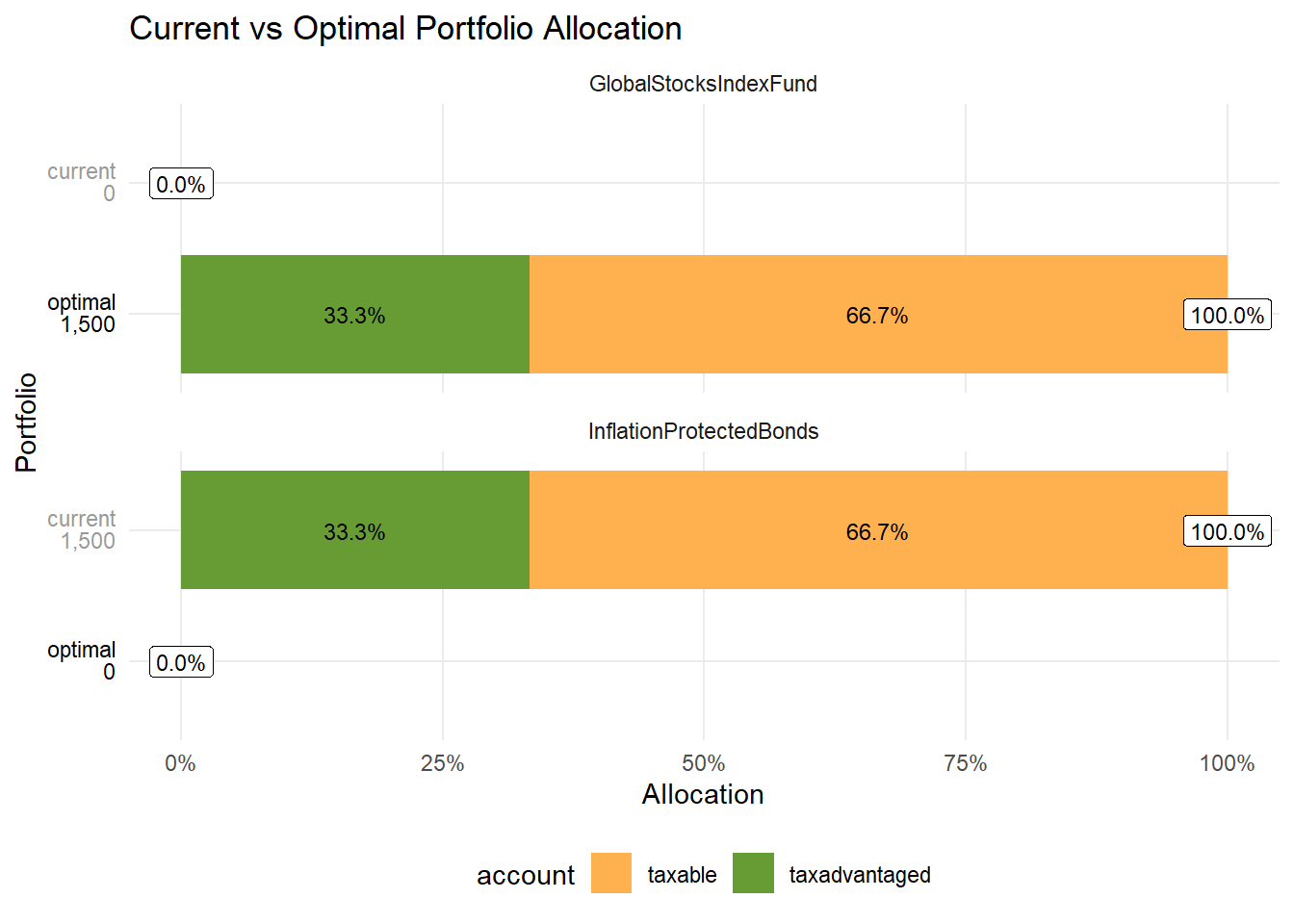
Juliet put all her savings—1’500 PLN—into inflation-protected bonds. But the optimal strategy for her seems to be to move everything into a global stock index fund or ETF, also using tax-advantaged accounts for that. Why? The next sections will reveal more.
The optimal asset allocation here is somewhat similar to the idea of optimal asset allocation based on Merton Share described in this post: How to Determine Our Optimal Asset Allocation?, but in this case, it also takes into account our lifetime human capital and liabilities.
Creating Household and Portfolio objects sets the stage to simulate various lifetime scenarios for Juliet.
Let’s start our simulations with the most basic scenario: we assume Juliet retires at age 60, and her portfolio performance is based on expected market returns.
scenario <-
  simulate_scenario(
    scenario_id  = glue::glue("Juliet retired at {retirement_start_age}"),
    household = household,
    portfolio = portfolio
  )
── Simulating scenario: Juliet retired at 60 ℹ Current date: 2025-01-01! Caching is NOT enabled.→ Simulating a scenario based on expected returns (sample_id==0)✔ Simulating a scenario based on expected returns (sample_id==0) [1.2s]To analyze the simulated data, let’s start by creating a table for Juliet with a scenario snapshot for a given year. Our table should capture values relevant to the current (first) year of our scenario simulation (when Juliet is 20 years old).
scenario |> render_scenario_snapshot(currency = "PLN")| Scenario Summary (2025) | |
|---|---|
| Scenario: Juliet retired at 60 | |
| Expected cashflow (monthly) | |
| Income | 4 995 PLN |
| Spending | 4 392 PLN |
| Non-discretionary spending | 3 500 PLN |
| Discretionary spending | 892 PLN |
| Savings | 603 PLN |
| Saving rate | 12.1% |
| Balance sheet | |
| Financial wealth | 1 500 PLN |
| Human capital | 1 823 314 PLN |
| Liabilities | 1 574 823 PLN |
| Net Worth | 249 992 PLN |
| Date: 2025-01-01 | |
Juliet finds actionable insights in the Expected cashflow section. Current assumptions suggest her optimal monthly discretionary spending is 892 PLN. Adding non-discretionary expenses, her total spending reaches 4’392 PLN. She needs to save monthly 603 PLN and invest it in her optimal portfolio.
Juliet’s balance sheet summary reveals the present values of three capital types:
Her net worth, calculated as the sum of financial and human capital minus liabilities, shows a positive value. This means her net worth could support discretionary spending. Although her financial assets are modest, her human capital—projected future income—offsets her life-time liabilities.
Juliet discovered the essential values from the scenario snapshot table. Let’s see how these values evolve over time.
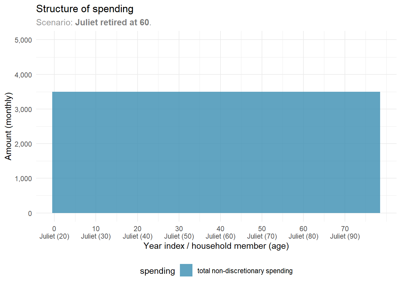
Let’s dive into Juliet’s future income and spending. We’ll start with her anticipated non-discretionary spending. This analysis is straightforward, as she has a single, consistent spending stream. It’s 3,500 PLN, adjusted for inflation, and remains steady over time.
y_limits <- c(NA, 5000)

scenario |>
  plot_future_spending(
    period   = "monthly",
    type     = "non-discretionary",
    y_limits = y_limits
  )
Let’s consider Juliet’s future expected income.
scenario |>
  plot_future_income(
    period   = "monthly",
    y_limits = y_limits
  )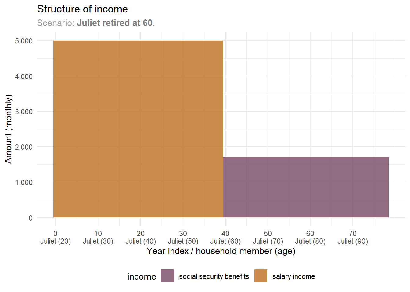
Her income includes two streams: salary and social security benefits. The salary stops when she retires at age 60. At that point, social security benefits kick in, as 60 is the earliest age women in Poland can claim. Currently, Juliet plans to start these benefits right after retiring.
We analyzed income and essential expenses. With this understanding, we can chart Juliet’s expected spending—discretionary and non-discretionary.
scenario |>
  plot_future_spending(
    period = "monthly",
    discretionary_spending_position = "top",
    y_limits = y_limits
  )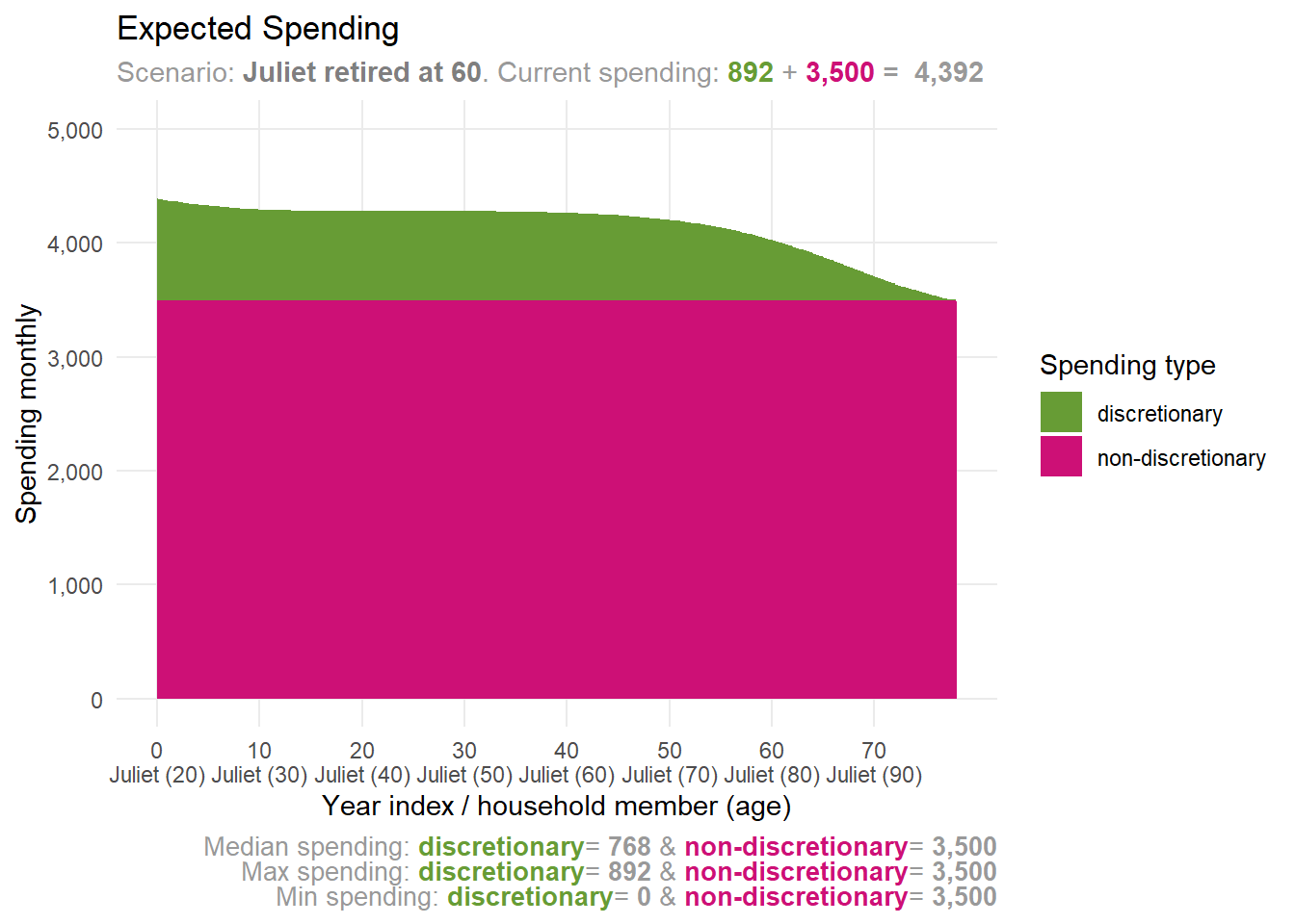
We’ve added discretionary spending on top of the non-discretionary spending plot. It starts at 892 PLN per month in the first year and then fluctuates. Why?
Several reasons: Discretionary spending hits zero as the chance of being alive drops. Meanwhile, Juliet’s household defaults to certain consumption preferences, showing a mix of consumption impatience and desire for smooth consumption. Each of these preferences shapes how discretionary spending changes over time. We are using some reasonable defaults here, but they can be adjusted to match Juliet’s preferences (Idzorek and Kaplan 2024, 17–20). We will discuss how to adjust these preferences in the later blog posts.
Right now, Juliet feels good about her future discretionary spending plans. She’s happy with the current setup, allowing her to indulge a bit more sooner rather than later.
Juliet’s savings are invested via both taxable and tax-advantaged accounts. Therefore, her spending should be seen as pre-tax. If she plans to cover her expenses with capital gains from taxable accounts, taxes need to be paid first. This means her true available spending will be lower.
Juliet wonders if her saving rate will remain steady, rise, or fall over time.
scenario |> plot_future_saving_rates()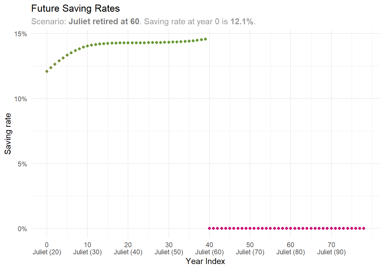
Juliet’s saving rates hover around 12% but are not flat. They stay relatively stable because her income and necessary spending remain steady. The key insight for Juliet is that her current saving rate isn’t permanent; it will likely increase over time as Juliet prefers to spend on non-discretionary items a bit more in the nearest future.
Juliet’s net worth is shaped by her human and financial capital, along with her liabilities. We can illustrate for Juliet how these elements are expected to change over time.
scenario |> plot_expected_capital()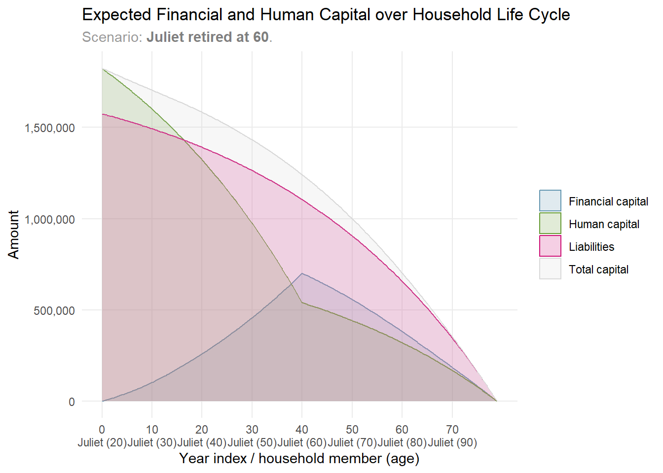
Juliet sees her human capital gradually transform into financial capital, covering both non-discretionary and discretionary expenses.
We’ve been looking at Juliet’s expected scenario, based on anticipated returns for her portfolio. But Juliet is aware that market returns carry uncertainty. Even with a fixed expected value and volatility, the order of those returns can impact Juliet’s finances negatively. This is known as the risk of sequence of returns.
Read more about the risk of sequence of returns in this section: Why is it important to account for the uncertainty of portfolio returns?
To address this, we can re-simulate Juliet’s scenario. We’ll generate not only the expected returns but also 500 Monte Carlo samples with varied sequences of random returns.
scenario <-
  simulate_scenario(
    household    = household,
    portfolio    = portfolio,
    scenario_id  = glue::glue(
      "Juliet retired at {retirement_start_age}"
    ),
    monte_carlo_samples = 500,
    seed                = 1234,
    use_cache           = TRUE,
    auto_parallel       = TRUE
  )
── Simulating scenario: Juliet retired at 60 ℹ Current date: 2025-01-01ℹ Setting random seed to 1234ℹ Generating random seeds for Monte Carlo samplesℹ Auto-parallelization enabled with 16 workers.ℹ Caching is enabled!→ Simulating a scenario based on expected returns (sample_id==0)✔ Simulating a scenario based on expected returns (sample_id==0) [1.8s]→ Simulating 500 Monte Carlo samples✔ Simulating 500 Monte Carlo samples [17.4s]Let’s revisit Juliet’s future discretionary spending. This time, we’ll compare her spending based on expected portfolio returns with spending predictions from various Monte Carlo simulations of potential return sequences.
scenario |> plot_future_spending("monthly", "discretionary")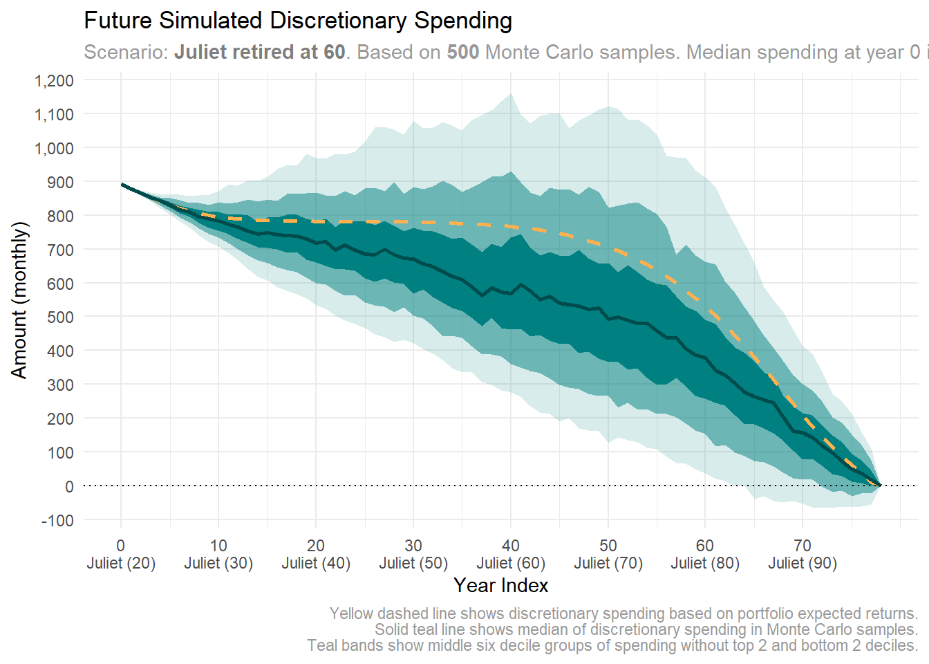
Juliet notices her discretionary spending shifts with portfolio returns, as shown in the plot. The median spending, marked by a solid dark teal line, drops faster than the expected spending, illustrated by a dashed yellow line. Yet, it remains above 500 PLN most of the time—sufficient in Juliet’s view.
If returns are unfavorable, Juliet can adapt. She might boost her savings, trim non-essential expenses, consider retiring later, or seek ways to increase her disposable income.
Juliet noticed that her future savings rate hovers below 15% when her portfolio sees expected returns. But how might these rates shift when averaged across multiple Monte Carlo samples with varying return sequences?
scenario |> plot_future_saving_rates()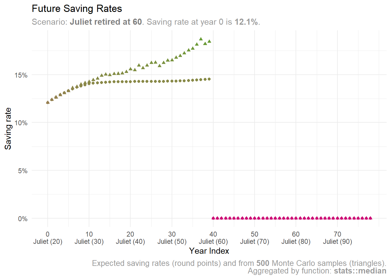
Triangles on the plot display median saving rates from all Monte Carlo samples. Juliet notices they’re rising over time, potentially exceeding 15% due to unfavorable portfolio sequence of returns.
If the worst-case scenarios unfolds, Juliet may need to adapt significantly. She might decide to retire later. Fortunately, she still has time to make that decision. For now, she can wait and assess the sequence of returns as they come, then make the best choice based on her current knowledge and future expectations.
Juliet wonders, what if she changes her retirement age? Can she retire a few years early and still maintain her lifestyle? Or, if she enjoys her work, could she continue longer and have more funds for her dreams?
Let’s create a set of parameters to explore Juliet’s options. We’ll examine retirement starting at ages 50, 55, 60, 65, and 70.
scenarios_parameters <-
  tibble::tibble(
    member    = "Juliet",
    event     = "retirement",
    start_age = seq(50, 70, by = 5),
    years     = Inf,
    end_age   = Inf
  ) |>
  dplyr::mutate(
    scenario_id = paste0(substr(member, 1, 1), "-", start_age)
  ) |>
  tidyr::nest(events = -scenario_id)

scenarios_parameters |>
  tidyr::unnest(events) |>
  print()
# A tibble: 5 × 6
scenario_id member event start_age years end_age
<chr> <chr> <chr> <dbl> <dbl> <dbl>
1 J-50 Juliet retirement 50 Inf Inf
2 J-55 Juliet retirement 55 Inf Inf
3 J-60 Juliet retirement 60 Inf Inf
4 J-65 Juliet retirement 65 Inf Inf
5 J-70 Juliet retirement 70 Inf Infscenarios <-
simulate_scenarios(
scenarios_parameters = scenarios_parameters,
household = household,
portfolio = portfolio,
use_cache = TRUE,
seeds = 1234
)After simulating multiple scenarios, let’s compare metrics for Juliet’s what-if scenarios on one plot.
scenarios |> plot_scenarios("monthly")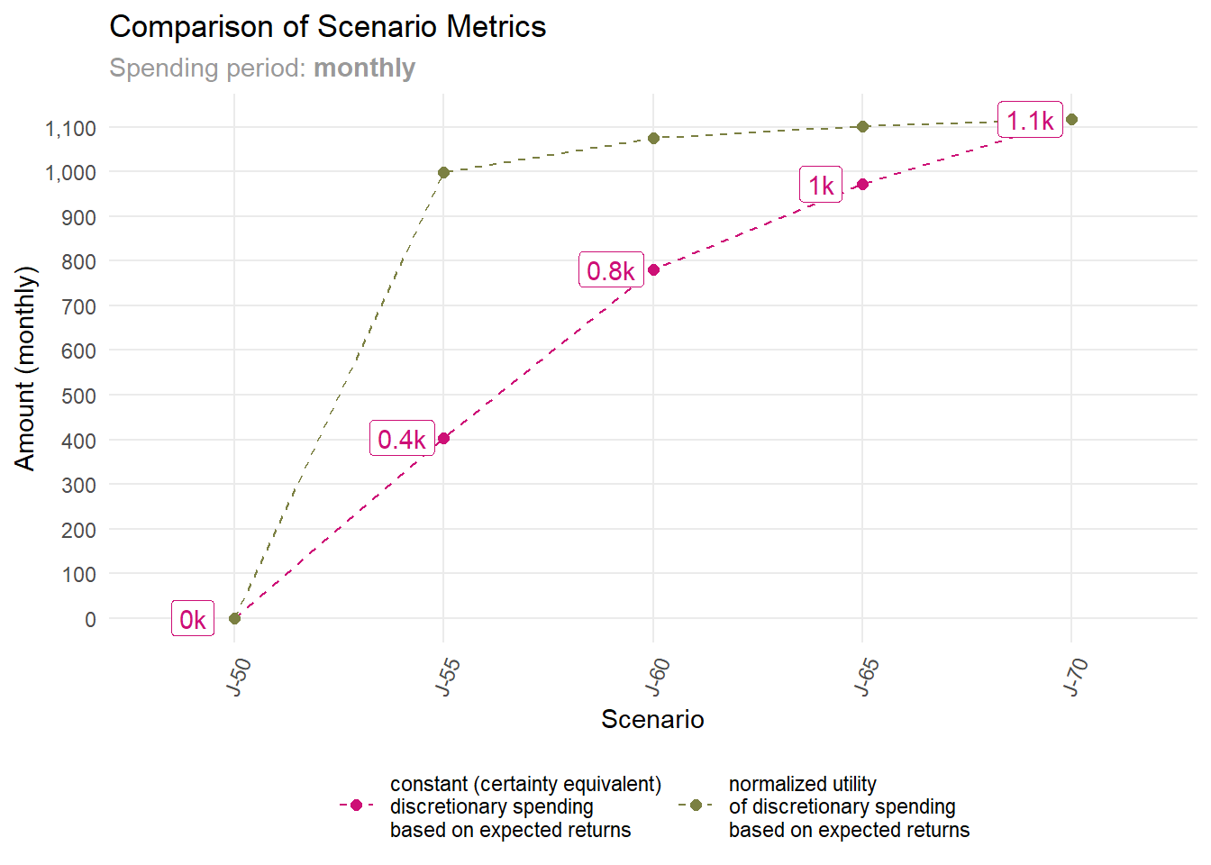
What this plot shows us? A key takeaway is that Juliet should consider scenarios offering notable metric gains.
Take retiring at 50, for example. In the “J-50” scenario (Juliet retiring at 50), her constant discretionary spending6 and normalized utility drop to zero. This means she’d lack enough capital for her expenses.
Now, consider retiring at 55. The “J-55” scenario shows a leap to nearly 400 PLN in constant discretionary spending, significantly boosting its utility.
What happens if she retires at 60, under the “J-60” scenario? Constant discretionary spending rises to around 800 PLN, but the utility gain isn’t as pronounced.
While later retirement slightly boosts discretionary spending utility, it still raises constant discretionary spending amount, though also at a slower rate.
Juliet sees 60 as her target retirement age. Yet, she’s curious about shifting the timeline. What if she retires five years earlier or later?
Juliet now wants to concentrate on two scenarios she finds most intriguing: retiring at the age of 55 or 65. This time, we plan to generate Monte Carlo samples to conduct a similar analysis to the one we did for the basic scenario (Juliet retiring at 60 years old). This will help us examine how the sequence of risk returns might impact these scenarios differently.
scenarios_parameters <-
  tibble::tibble(
    member    = "Juliet",
    event     = "retirement",
    start_age = c(55, 65),
    years     = Inf,
    end_age   = Inf
  ) |>
  dplyr::mutate(
    scenario_id = paste0(substr(member, 1, 1), "-", start_age)
  ) |>
  tidyr::nest(events = -scenario_id)

scenarios <-
  simulate_scenarios(
    scenarios_parameters = scenarios_parameters,
    household            = household,
    portfolio            = portfolio,
    monte_carlo_samples  = 200,
    use_cache            = TRUE,
    auto_parallel        = TRUE,
    seeds                = 1234
  )
Let’s compare Juliet’s what-if scenarios. We’ll begin with differences in future discretionary spending.
Juliet wonders how retiring at 55 might affect her discretionary spending.
y_limits <- c(NA, 1500)
scenarios |>
  dplyr::filter(scenario_id == "J-55") |>
  plot_future_spending("monthly", "discretionary", y_limits = y_limits)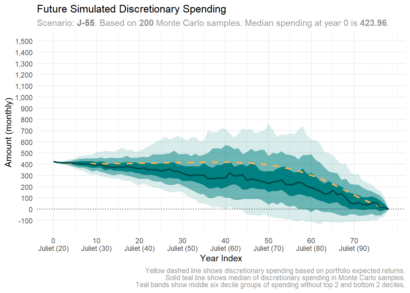
Juliet’s early retirement plan requires her to cut discretionary spending to 423 PLN. There’s also a heightened risk of depleting her capital if returns falter.
She’s considering now waiting until the age of 65 to retire. Could this boost her future spending potential?
scenarios |>
  dplyr::filter(scenario_id == "J-65") |>
  plot_future_spending("monthly", "discretionary", y_limits = y_limits)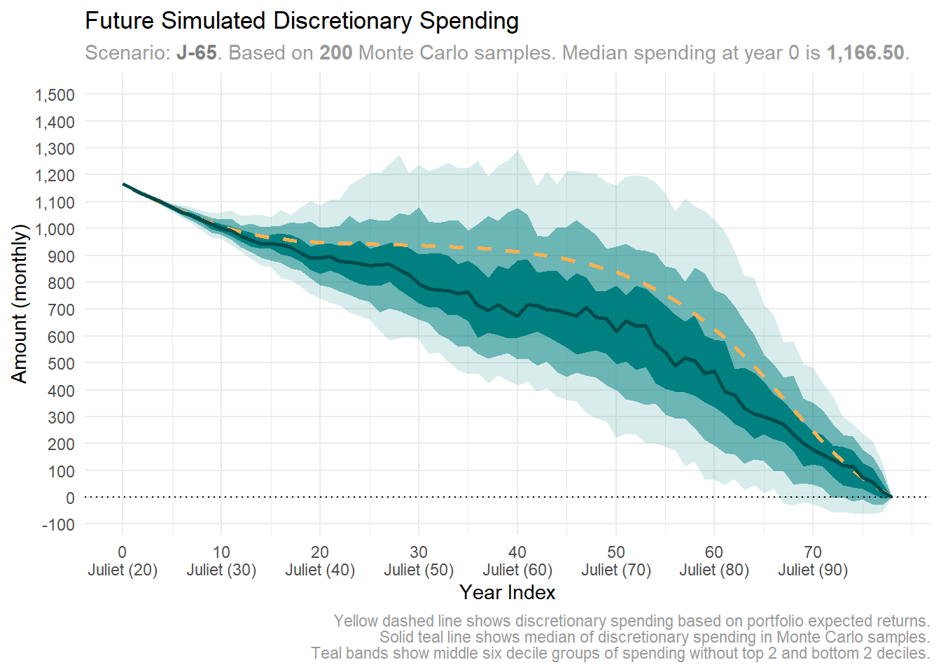
If Juliet retires at 65, she can begin spending 1,166 PLN on discretionary items. Even with less favorable returns, she likely has enough capital to cover additional discretionary spending in the hundreds.
How might these scenarios affect Juliet’s future saving rate?
Juliet wonders how her saving rates would look if she retires at various ages.
y_limits <- c(NA, 0.25)

scenarios |>
  dplyr::filter(scenario_id == "J-55") |>
  plot_future_saving_rates(y_limits = y_limits)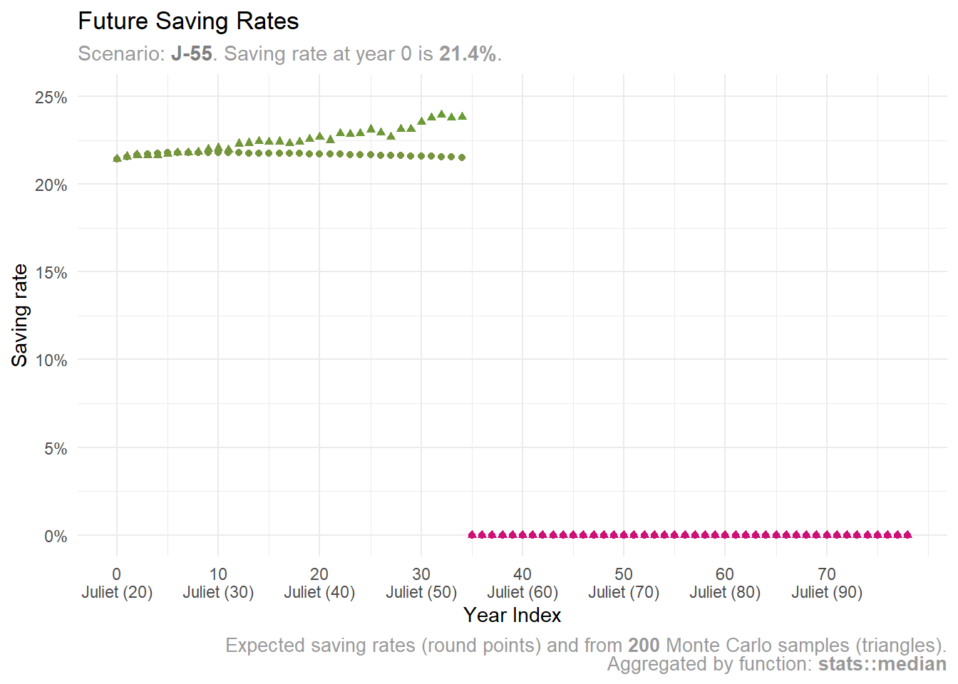
Juliet realizes she needs to save more—over 20%—if she wants to retire early at 55.
scenarios |>
  dplyr::filter(scenario_id == "J-65") |>
  plot_future_saving_rates(y_limits = y_limits)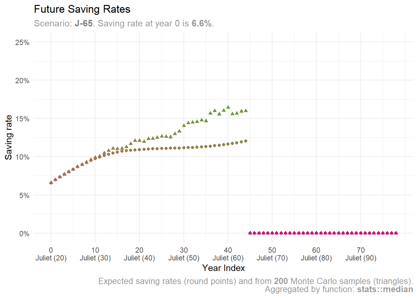
If Juliet retires at 65, she might need to save less—under 10%. However, she may need to boost savings if return rates aren’t favorable.
Juliet’s final focus is on tracking how her optimal asset allocation changes across various retirement scenarios.
scenarios |>
  dplyr::filter(scenario_id == "J-55") |>
  plot_expected_allocation()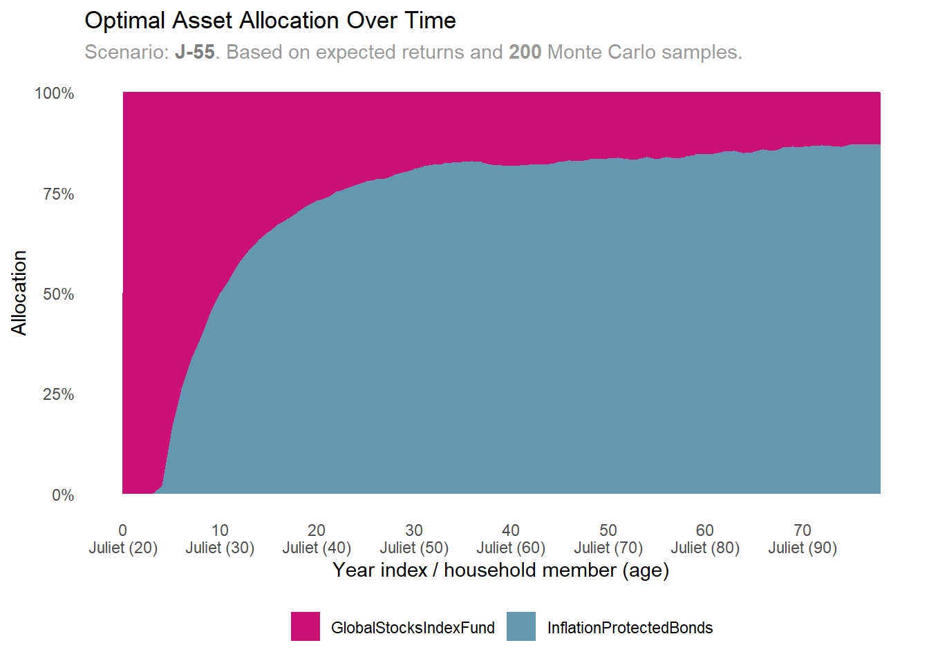
scenarios |>
  dplyr::filter(scenario_id == "J-65") |>
  plot_expected_allocation()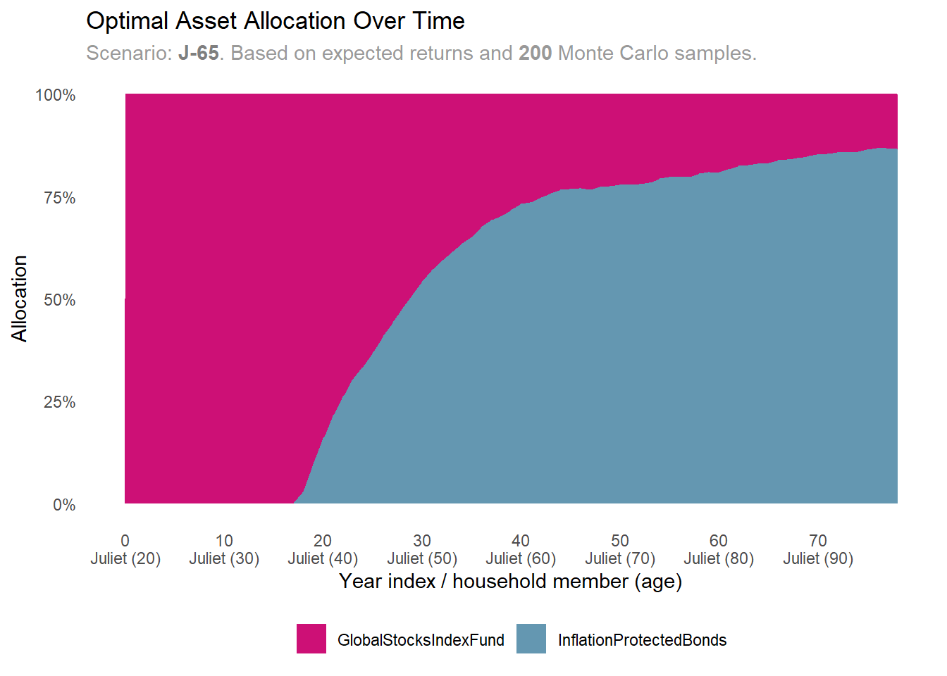
In both retirement scenarios, the model advises Juliet to invest all her financial capital in stocks. This makes sense because her small financial capital is offset by significant bond-like human capital.
As time progresses, the model recommends moving towards bonds in both scenarios. However, in the later retirement scenario, the shift to stocks occurs later than in the earlier one. This is because Juliet plans to work longer, maintaining a larger human capital that she will convert into financial capital over an extended period.
There are several ways in which Juliet can decide to extend the lifecycle model and simulations:
We assumed Juliet will only claim the minimum social security benefits at retirement. That may be too pessimistic. Even if the average pension replacement rate for young people like Juliet in Poland might be around 40% (OECD 2023, 53–54), Juliet could still receive roughly 2,000 PLN per month at age 60 in today’s terms. That’s a bit more than the current minimum social security benefits (1,710).
Moreover, Juliet’s social security pension will grow if she waits before claiming it. Delaying each year boosts her pension by 8-10% 7. Waiting for 10 years, until age 70, could increase Juliet’s pension to 4,000 PLN or more.
Should Juliet delay claiming Social Security? That is a topic for another post. But it’s worth considering in her financial model. Social Security works like an inflation-indexed annuity from the recipient’s perspective (Ibbotson et al. 2007, vii). This makes it crucial insurance against outliving ones savings.
Juliet thrives solo in a single-person household in a bustling Polish city. She navigates life independently, whether or not Romeo is by her side, or if they haven’t crossed paths, or perhaps they did, but he wasn’t quite right for her. Our simulations suggest this single-person household scenario is realistic for Juliet.
Juliet bases her decisions on current assumptions about the future market and a median salary that aligns with inflation. The future is uncertain, which means these assumptions might shift. However, decisions must be made today, rooted in what seems most reasonable right now.
When the future looks bleak, Juliet will adapt. She might ramp up her savings, cut unnecessary costs, think about retiring later, or find ways to boost her income—like taking on part-time work or seizing business opportunities. But if the future shines bright, she could decide to enjoy more discretionary spending, retire earlier, or even do both.
You can see that with the household lifecycle framework you can quite quickly reach an optimal (or near-optimal) recommendation tailored to your own specific situation at a given moment.
In future posts, we’ll explore scenarios where Juliet and Romeo choose to spend their life together. Our simulation will include diverse income sources, multiple necessary expenses, and varied life expectancy assumptions. Eventually, we’ll even factor in children.
Enjoyed this post? Share it with others who might find it interesting. Subscribe to our newsletter to stay updated. Thanks for reading!
Juliet’s expectation for clear advice seems to be in line with the Financial Planning Competency Handbook by the CFP Board: Presenting planning alternatives, while useful in showing a client the many paths available to reach a financial goal, can create decision paralysis among some clients. This is the reason that the planner should conclude with a clear set of recommendations that leave the client in no doubt as to what must be done next (CFP Board 2015, 606). Using life-cycle model, we can recommend Juliet not only one of many alternatives of recommendations, but a single set of recommendations that should be optimal for her (or at lest close to optimal).↩︎
The median salary in Poland in 2024 was 6’842 PLN gross per month, and about 4’995 PLN net per month. See: https://stat.gov.pl/obszary-tematyczne/rynek-pracy/pracujacy-zatrudnieni-wynagrodzenia-koszty-pracy/rozklad-wynagrodzen-w-gospodarce-narodowej-w-listopadzie-2024-r-,32,11.html↩︎
The net minimum social security benefits in Poland in 2025 is 1’878.91 PLN per month gross, which is about 1’709.81 PLN net. See: https://www.gov.pl/web/rodzina/waloryzacja-rent-i-emerytur-w-2025-roku–wzrost-swiadczen-dla-milionow-polakow↩︎
The costs of leaving for a single in a big city in Poland in 2025 were estimated at 4’000 PLN per month. This included also discretionary spending like 450 PLN for cinema tickets, eating out, subscriptions. Based on that we assumed that non-discretionary spending is about 3’500 PLN. See: https://www.bankier.pl/smart/ile-kosztuje-zycie-singla-vs-rodziny-w-2025-budzety-ktore-otwieraja-oczy (in Polish)↩︎
Read more about human capital in (Milevsky 2012), (Ibbotson et al. 2007), and (Idzorek and Kaplan 2024).↩︎
Constant discretionary spending—certainty equivalent constant level of spending that would result in the same lifetime utility as a series of (non-constant) future spending in a given scenario.↩︎
See article (in Polish): https://businessinsider.com.pl/praca/emerytury/emerytura-jak-uzyskac-wyzsze-swiadczenie-ike-ppk-odroczenie-emerytury-prezes-zus/cx88knm. The similar situation is in US, where Social Security payments increase 8 percent for every year after full retirement age that a retiree waits to claim benefits. A retiree who des not take early Social Security benefits may enjoy a benefit up to 30 percent grater than one who receives benefits at the earliest possible age. (CFP Board 2015, 437)↩︎
@online{wais2025,
  author = {Wais, Kamil and Wais, Olesia},
  title = {Can {Juliet} Manage Without {Romeo?} {How} Much She Should
    Spend, Save, and Invest to Achieve That?},
  date = {2025-07-27},
  url = {https://r4good.academy/en/blog/financial-report-individual-minimal-example/index.en.html},
  langid = {en}
}