Why and How to Calculate Retirement Ruin Probability?
You will learn why so called Safe Withdrawal Rates (SWR) might not be reliable. You will understand the importance of considering the uncertainties of our lifespan and portfolio returns. You will learn what retirement ruin probability is, how to calculate it, and when to apply it while being aware of its limitations.
R4GoodPersonalFinances
R package
RBloggers
Personal Finances
retirement
withdrawal rates
Safe Withdrawal Rate
SWR
survival rates
Gompertz model
Authors
Kamil Wais
Olesia Wais
Published
April 19, 2025
What will you learn from this article?
Jorge Guinle—the famous Brazilian playboy—died on Friday the fifth of March 2004 in Rio de Janeiro. Jorge was born to one of the wealthiest families in Brazil, and he spent a large part of his life dating famous Hollywood starlets such as Rita Hayworth, Lana Turner, and Marilyn Monroe. This hobby was quite expensive and apparently he squandered most of his family’s fortune well before he died at the age of 88. In fact, in an interview a few years before his death, Jorge said: “The secret of living well is to die without a cent in your pocket. But I miscalculated, and the money ran out too early.” (Moshe A. Milevsky 2006, 185).
The quote above is from the book “The Calculus of Retirement Income” (Moshe A. Milevsky 2006, 185), written by Moshe Milevsky. He authored other notable books and papers, and introduced the retirement ruin metric. His work inspired us to write this post. Here, you’ll learn insights that could have helped Jorge with essential calculations, improved his financial decisions, and prevented his funds from running out too soon. It is too late for him, but maybe you have found us at the right time. You will also discover why we should be cautious about blindly trusting everything popular influencers recommend.
From this article you will learn:
What does the initial withdrawal rate refer to, and why is it often termed the Safe Withdrawal Rate (SWR) even when it isn’t really safe?
Why is it crucial to consider the uncertainty of our lifespan and portfolio returns?
What does retirement ruin probability mean?
How is the retirement ruin probability calculated?
Why are metrics based on a constant (real) withdrawal rate typically are poor foundation for decision making?
In what situations could retirement ruin probability still be useful?
Tip
All calculations and plots in this article are done with the use of the functions from the R4GoodPersonalFinances R package:
The Safe Withdrawal Rate (SWR) is a well-known concept among individuals preparing for retirement. Its goal is to establish an annual spending amount that ensures you won’t deplete your savings within your lifetime. However, this concept has several issues. Let’s explore what the SWR truly entails and evaluate its actual safety with the retirement ruin framework.
What is the Safe Withdrawal Rate (SWR)?
People are often convinced that a safe withdrawal rate is around 4%. What does this imply? It suggests that if you retire this year, you can initially withdraw 4% of your investment portfolio in the first year. In the years that follow, you can withdraw the same amount, adjusted for inflation.
The initial withdrawal rate determines the amount you can spend each year for… exactly how long? The Safe Withdrawal Rate suggests that your annual withdrawals should sustain you throughout your lifetime. But let’s briefly address issues that can arise from using the Safe Withdrawal Rate as a single and universal figure to determine your withdrawal amount per year.
For a 4% widthrawal rate to be considered safe, there are many assumptions and questions about your portfolio’s returns that are hidden and factors that can result in the success or failure of your retirement plan: At what age are you planning to retire? How long is your lifespan expected to be? For how many years should your savings last? What if you live significantly longer than anticipated? What happens if your investment portfolio underperforms or outperforms expectations?
From these questions, we see that the SWR is an oversimplified metric acting as a one-size-fits-all solution. That’s why it’s crucial to consider other, more comprehensive metrics of retirement planning. The retirement ruin probability is one of them.
What is the retirement ruin probability?
The lifetime probability of ruin serves as a risk metric to determine if our planned withdrawal rate is too risky.
Like the SWR approach, we assume we’ll withdraw and spend the same inflation-adjusted amount annually for the rest of our lives. It’s crucial to note that this amount is before income taxes, meaning the disposable amount will be lower post-tax.
In this context, “ruin” refers to depleting one’s personal resources, such as an investment portfolio (Moshe A. Milevsky and Robinson 2005, 90–91). This situation is commonly known as the “failure rate,” in contrast to the “success rate.”
Similar to real (inflation-adjusted) spending, we define our portfolio returns in terms of real (inflation-adjusted) annual returns. We also use the standard deviations of these returns to measure their volatility.
Unlike with SWR, we accept that both our lifespan and portfolio returns are random variables. We may have some expectations about these, but their actual outcomes remain uncertain. This approach contrasts sharply with the assumption that our portfolio will yield a fixed annual return of X percent or that we will live precisely Y years in retirement.
When it comes to our lifespan, it is also not as simple as checking the current life expectancy of people in your country for calculating how many years you’ll have in retirement. If you hear that the current life expectancy in your country is 80 years and you’re retiring at 65, you shouldn’t plan for just 80 - 65 = 15 years. As Moshe Milevsky noted:
“Although the oft-quoted statistic for life expectancy is somewhere between 78 and 82 years in the United States, this statistic is relevant only at the time of birth. If pensioners reach their retirement years, they may be facing 25-30 more years of life with substantial probability because conditional life expectancy increases with age […] The aim is not to guess or take point estimates, but, rather, to actually account for this uncertainty within the model itself (Moshe A. Milevsky and Robinson 2005, 91–92).
Note
For those more inclined to math, the lifetime probability of ruin uses the concept of stochastic present value (SPV), which is a random variable with a probability density function (PDF) that depends on the risk-return parameters of the underlying investment-generating process and the random future lifetime. If the SPV of the consumption plan is probabilistically larger than the current portfolio value, then the retirement plan is unsustainable and the individuals will be “ruined” at some point, unless, of course, they reduces consumption (Moshe A. Milevsky and Robinson 2005, 92, 94).
Why is it worth calculating retirement ruin probability?
Using retirement ruin probability, we can quickly assess whether our initial withdrawal rate appears safe (with a ruin probability close enough to zero). Simultaneously, the retirement ruin probability takes into account the uncertainty and variability of both our portfolio returns and our lifespan.
We could achieve similar outcomes through Monte Carlo simulation; however, calculating retirement ruin probability is quicker and easier than conducting complex simulations involving multiple random variables. It has been shown that the “results are remarkably accurate when compared with more costly and time-consuming simulations” (Moshe A. Milevsky and Robinson 2005, 90). Thus, using retirement ruin probability provides a sufficiently good approximation when compared to Monte Carlo simulations (Moshe Arye Milevsky and Robinson 2000, 119).
We mentioned that it’s important to consider the uncertainty of our lifespan. Why is that? Can’t we simply assume we’ll live to a certain age?
Why is it important to account for lifetime uncertainty?
The maximum human lifespan is currently about 120 years. This implies that a 65-year-old could potentially spend 55 years in retirement. That equates to another half-century of relying on savings accumulated in the earlier years.
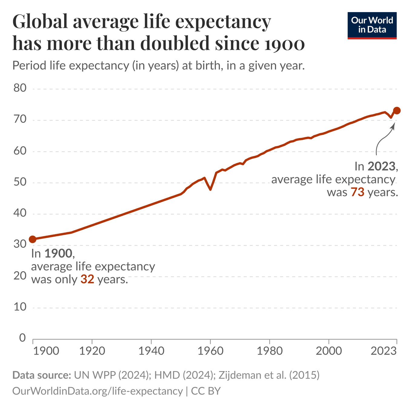
It’s true that some of us might live to an advanced age, yet this represents only a tiny fraction of the population. Most will have a shorter life expectancy. However, life expectancy is gradually rising. Since 1900, the global average life expectancy has more than doubled, reaching 73 years in 2023 (See Figure 1).
Figure 1: Changes in global average life expectancy
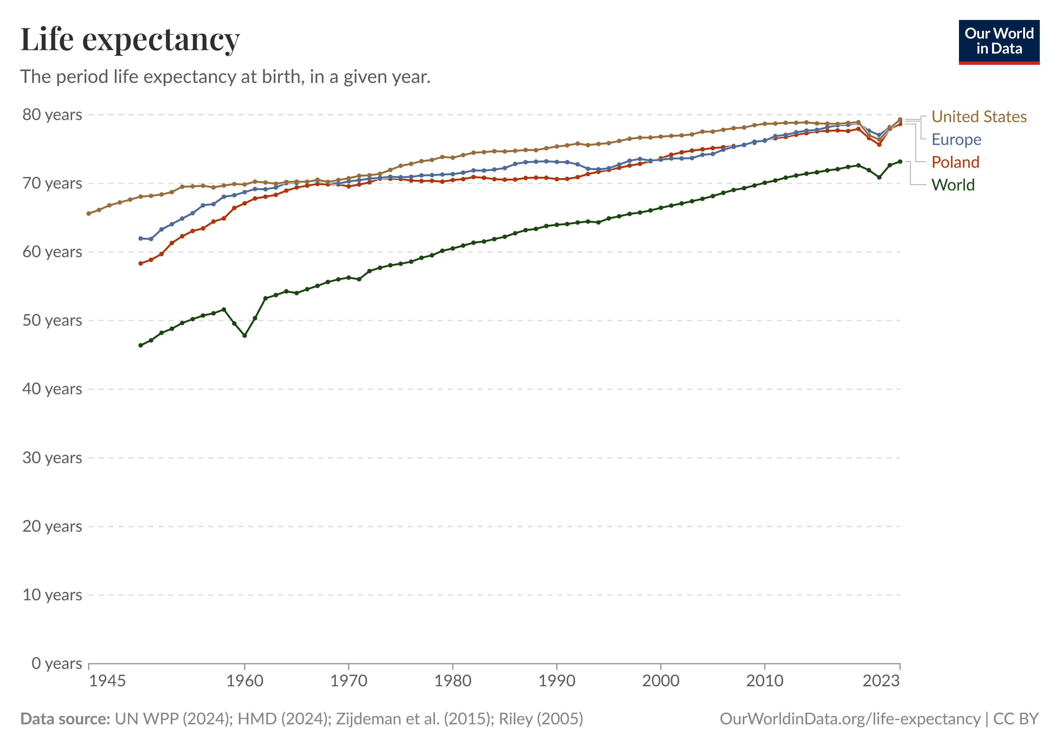
Furthermore, people in every region of the world today can expect to live more than twice as long as in the past.(Roser 2018)In the US and Europe, the average life expectancy reached nearly 80 years in 2023. (See Figure 2).
Figure 2: Comparing changes in life expectancy
Rather than slowing down, recorded life expectancy has been rising steadily over time, by around one year every four years. In some places, it has even reached 88 years (such as in Hong Kong in 2021). (Roser 2020)
As human population continues to experience increased longevity, we inevitably spend more years in retirement. While this is beneficial, it also poses challenges to many modern retirement systems and shifts the responsibility of retirement planning onto individuals like us. Consequently, we must plan for situations where we might not reach the average life expectancy, as well as for situations where we might significantly exceed it.
Why is it important to account for the uncertainty of portfolio returns?
Apart from the uncertainty of our lifespan, we also have to account for the uncertainty of our portfolio’s returns.
When you rely on a single number to represent your portfolio’s expected annual return, it’s easy to overlook the fact that actual returns can vary each year.
Consider a simplified example where we invest a portfolio of $100 in stocks for four years, experiencing returns that range from highly positive to highly negative.
Now, let’s examine what happens to our portfolio value at the end of the fourth year if we only buy and hold $100, without withdrawing from the portfolio to cover any expenses.
After four years, our portfolio is valued at $112. Let’s keep this figure in mind.
Now, let’s consider what occurs if the sequence of returns is reversed. You would initially face very negative returns, followed by very positive ones.
After four years, the portfolio value remains at $112, which is good news. If there are no withdrawals from the portfolio, and we can keep holding our stocks, the sequence of returns becomes irrelevant. We simply need to wait patiently for better years.
Beware of the risk of the sequence of returns!
Now things are getting intriguing. Let’s examine the outcome if we choose to retire and annually withdraw $20 from our portfolio to cover expenses.
If the sequence of returns starts positively, we’re in a good position. Although our portfolio’s value decreases, we still have a substantial amount left after four years to cover additional spending.
Now, we lack the funds to cover our expenses in the fourth year! We’re in a dire situation!
Important
If you’re withdrawing from the portfolio, the sequence of returns is crucial. Negative returns early on are more harmful than those occurring later. This is called the “risk of the sequence of returns”.
Please note that, in this simplified case, the expected annual return is positive and approximately 2.9%. However, the expected annual return does not provide any insight into the sequence of potential returns.
It is crucial to consider not only the expected yearly return of your portfolio but also the many possible scenarios of different return sequences. The returns will be volatile if your portfolio includes stocks. Some sequences of returns might be favourable, while others could work against you, raising the risk of your retirement ruin.
How to calculate retirement ruin probability?
To calculate your personal retirement ruin probability, you must prepare several inputs for the calc_retirement_ruin() function:
First, provide the age at which your retirement begins. If you wish to determine if you can retire immediately, use your current age.
Next, determine your desired monthly spending in real (inflation-adjusted) pre-tax dollars during retirement.
Also, provide the value of your investment portfolio at the start of the retirement.
As you want to account for uncertainty in portfolio returns, you’ll need two parameters to describe the distribution of annual returns: the mean and the standard deviation.
Lastly, to account for the uncertainty regarding your lifespan and years in retirement, it’s essential to specify two additional parameters of the Gompertz mortality distribution: the mode and the dispersion.
How do we obtain those parameters? We’ll begin by discussing how to model our probability of survival.
How to model our probability of survival?
Survival rates can vary greatly across different populations. For example, a 65-year-old’s chance of living to 80 depends heavily on the country they live in. It also varies by gender, whether the person is male or female. Age plays a role too; if someone lives to 70, their probability of reaching 80 increases, given they have already reached 70. Additionally, when considering two adults in a household, and we want to ensure that our retirement remains secure as long as one of them is alive, we should examine their joint survival probabilities.
To address all these factors, we will begin by fitting the Gompertz model to population data. Following this, we will calibrate it to each individual and, finally, to the joint survival of a couple. However, let’s first explain what the Gompertz’s survival probability is.
What is Gompertz’s survival probability?
Benjamin Gompertz discovered that our probability of dying in the next year increases by approximately 9% per year, from adulthood until old age. So in other words, your mortality rate increases by something between 8% and 10% per year, with the average being about 9% (Moshe A. Milevsky 2012).
In the Gompertz model, the distribution of survival probabilities is characterized by two parameters: mode and dispersion. The mode indicates the peak of the distribution, while dispersion describes how spread out the values are around the mode.
If we average the numbers across all countries, we can agree on some global parameters. For instance, the global modal value is around 88 years, and the dispersion is about 10 years. However, there is considerable variation between countries (Moshe Arye Milevsky 2020, 266).
For now, let’s use these global parameters to determine the Gompertz probability of surviving to age 85, starting from the time of birth.
Code
surv_prob<-calc_gompertz_survival_probability( current_age =0, target_age =85, mode =88, dispersion =10)surv_prob|>print_percent(prefix ="Probability of surviving from birth to age 85: ")
[1] "Probability of surviving from birth to age 85: 47.7%"
The probability of surviving to age 85 from birth is 47.7%. Let’s assume this individual has now reached the retirement age of 65.
Code
surv_prob<-calc_gompertz_survival_probability( current_age =65, target_age =85, mode =88, dispersion =10)surv_prob|>print_percent(prefix ="Probability of surviving from age 65 to 85: ")
[1] "Probability of surviving from age 65 to 85: 52.7%"
The probability of surviving to 85 years old at the time of retiring at 65 is 52.7%. Thus, the probability has increased slightly.
Now, let’s assume this person has reached the age of 80.
Code
surv_prob<-calc_gompertz_survival_probability( current_age =80, target_age =85, mode =88, dispersion =10)surv_prob|>print_percent(prefix ="Probability of surviving from age 80 to 85: ")
[1] "Probability of surviving from age 80 to 85: 74.7%"
The probability of surviving to 85 years, given that one has already reached 80 years, is 74.7%. This shows that the chance of reaching age 85 increases with age.
The challenge is to adjust (calibrate) the Gompertz model parameters (mode and dispersion) to your specific situation or at least to the subpopulation you belong to. This ensures that the model accurately reflects your own survival probability rather than those of a general global population, which may have significantly different characteristics.
The classic Gompertz mortality function, when properly calibrated, is an excellent approximation for mortality, particularly at retirement ages(Moshe Arye Milevsky and Robinson 2000, 114). However, it poorly represents mortality at younger ages, under 30 years (Moshe Arye Milevsky 2020, 141). This isn’t an issue for us, as our focus is on later retirement years.
To calibrate the model to the population you are a part of, we need to find some data to fit the model. Fortunately, such data are easily available for everybody.
Calibrating the Gompertz model to our population
Finding the right data that we can use for calibration
The Human Mortality Database (HMD) is the world’s leading scientific data resource on mortality in developed countries. It is maintained by the Department of Demography at the University of California, Berkeley, the Max Planck Institute for Demographic Research, and the French Institute for Demographic Studies Mortality Research. More importantly, detailed data for many (40+) countries are available for free (after registration). They are also standardized to a common format and updated if new data are available for a given country. (Human Mortality Database 2025) Also available for each country are the life tables for females, males, and both sexes, so we can use data from more precisely defined populations where we fit most.
After obtaining the data for our population, we need to determine the Gompertz model parameters (mode and dispersion) that best align with this data. Technically, this involves fitting a Gompertz distribution to a discrete mortality table across various initial ages, using a nonlinear optimization algorithm (Moshe Arye Milevsky and Robinson 2000, 114–15) to identify appropriate Gompertz parameters (D. M. Blanchett and Kaplan 2013, 19–20).
In the R4GoodPersonalFinances R package, you can access mortality rates for the USA and Poland without needing to download or import the data manually. If you want us to include data for additional countries, please let us know.
The life_tables object from the package is a long data frame with column mortality_rate for a given year, age, sex and country. Let’s find the most recent mortality rates available, for females living in the USA.
# A tibble: 6 × 6
  country sex     year   age mortality_rate life_expectancy
  <chr>   <chr>  <int> <int>          <dbl>           <dbl>
1 USA     female  2022     0        0.00512            80.3
2 USA     female  2022     1        0.0004             79.7
3 USA     female  2022     2        0.00024            78.7
4 USA     female  2022     3        0.0002             77.7
5 USA     female  2022     4        0.00015            76.8
6 USA     female  2022     5        0.00014            75.8
Calculating parameters and checking model calibration
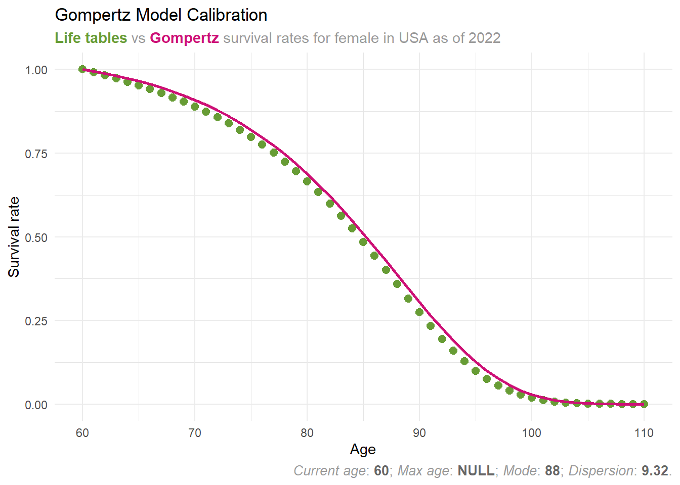
The filtered mortality rates are input into the calc_gompertz_parameters() function to determine the Gompertz parameters. Remember, we also need to set the current age of the person in question, as the survival probabilities depend on the person’s current age.
The Gompertz survival rates (shown in red) closely match the values derived from life tables (displayed in green). Thus, with these two parameter values, we can effectively predict the survival probabilities of an average 60-year-old female from the USA.
The model calibration was successful this time, though it isn’t always effective. When it falls short, we attempt to address the issue by using a modified Gompertz function.
Truncated version of Gompertz function for the rescue
We noted that the Gompertz model struggles to accurately represent the survival of very young individuals. Moreover, it faces another challenge at the opposite end: modeling the survival of very old individuals, such as centenarians. Something intriguing begins to occur once a person surpasses the age of 100.
Moshe Milevsky described it nicely: “[…] when mortality tables are compiled for people who died at age 100 and beyond, something remarkable shows up in the data. The mortality rate doesn’t increase by 9%, 5%, or 1% per year. It stops increasing altogether! The mortality rate flattens somewhere around 104, and the odds of dying in the next year plateau at about 50%. It doesn’t change from year to year. Basically, after the age of 105 or so, it becomes a coin toss” (Moshe A. Milevsky 2012).
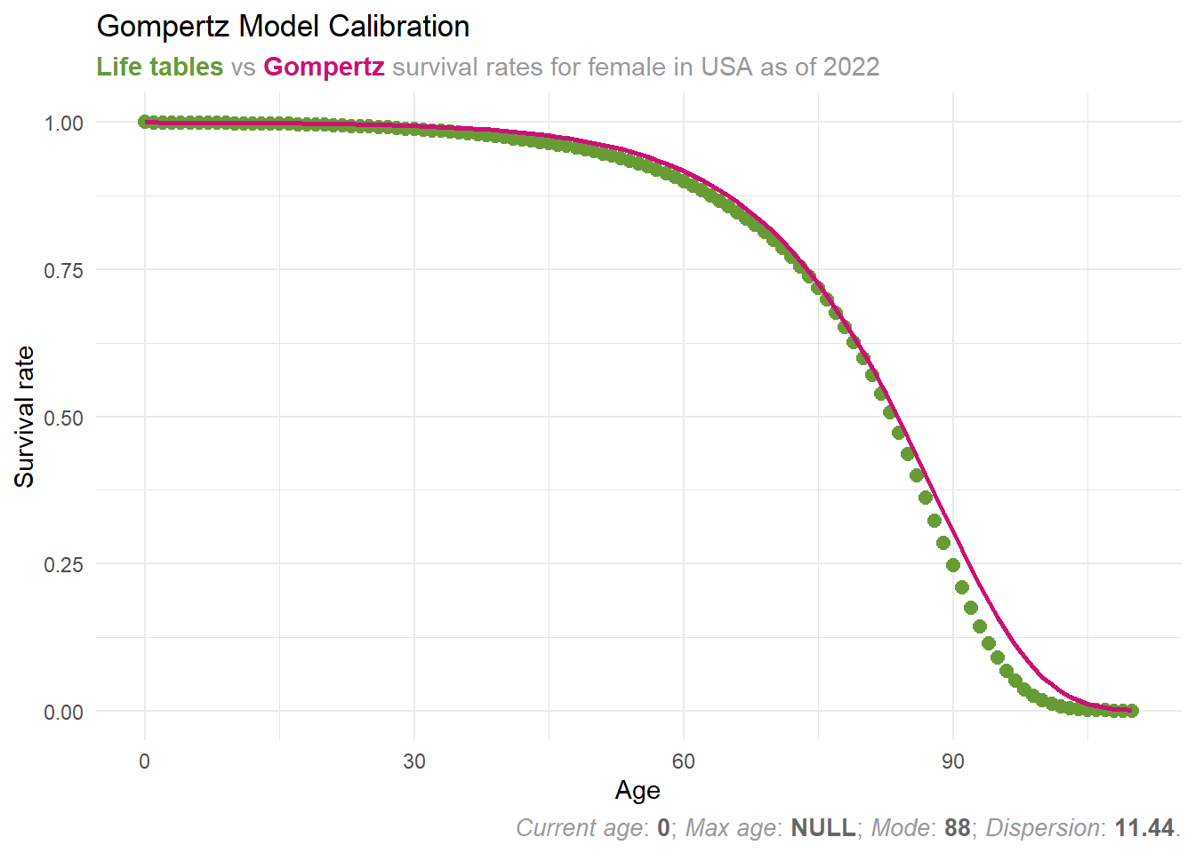
Let’s demonstrate how these modeling challenges affect our Gompertz model and explore potential solutions. Let’s attempt to calibrate the Gompertz parameters for a new-born female in the USA and examine her lifetime survival probabilities.
Our Gompertz (red) line appears to be poorly fitted, particularly for survival probabilities beyond 90 years. This can be adjusted using a workaround suggested by Thomas Idzorek and Paul Kaplan, involving the “truncated Gompertz function” (Idzorek and Kaplan 2024, 57–59, 63–64).
By implementing this approach, we determine a maximum age where we cease considering survival probabilities. We assume these probabilities are so minimal that we effectively treat them as zero.
The authors handle the truncation point as a manually chosen arbitrary value. However, in our approach, we concurrently fit it alongside the dispersion parameter using our optimization algorithm. Additionally, we ensure that survival probabilities beyond the maximum age point are zero, avoiding negative values.
Let’s examine our calibration when we also estimate the max_age parameter.
Once more, our Gompertz model survival curve appears to fit the data well. For simplification, we will not use the truncated Gompertz function further in this post. However, it will be useful when we advance to more complex life-cycle modeling.
We know how to apply the Gompertz model to population data and adjust it to represent an average individual within that population. But how do we tailor it to fit our specific situation?
Calibrating the Gompertz model to our individual situation
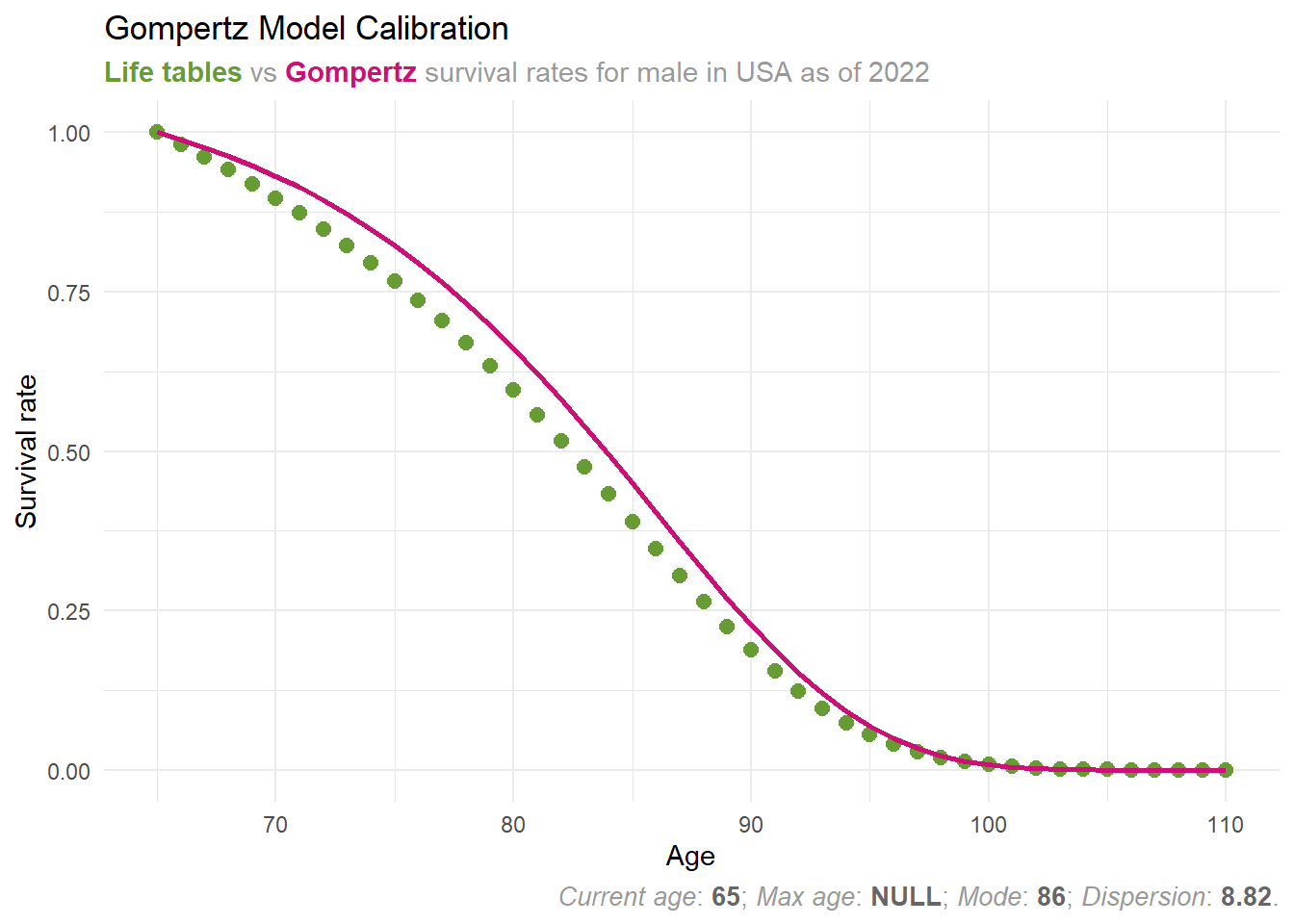
We will begin by calibrating the Gompertz model for a 65-year-old man in the USA. As previously, we’ll use available mortality rates to fit the model parameters.
The Gompertz model appears overly optimistic about survival rates compared to actual data. We can attempt to adjust it, but let’s consider the scenario of a man in excellent health. He has no diseases, maintains good lifestyle habits, follows a plant-based diet, engages in regular daily physical activity, and comes from a family with a history of longevity. Everything suggests he should have higher survival probabilities than the average male in his population.
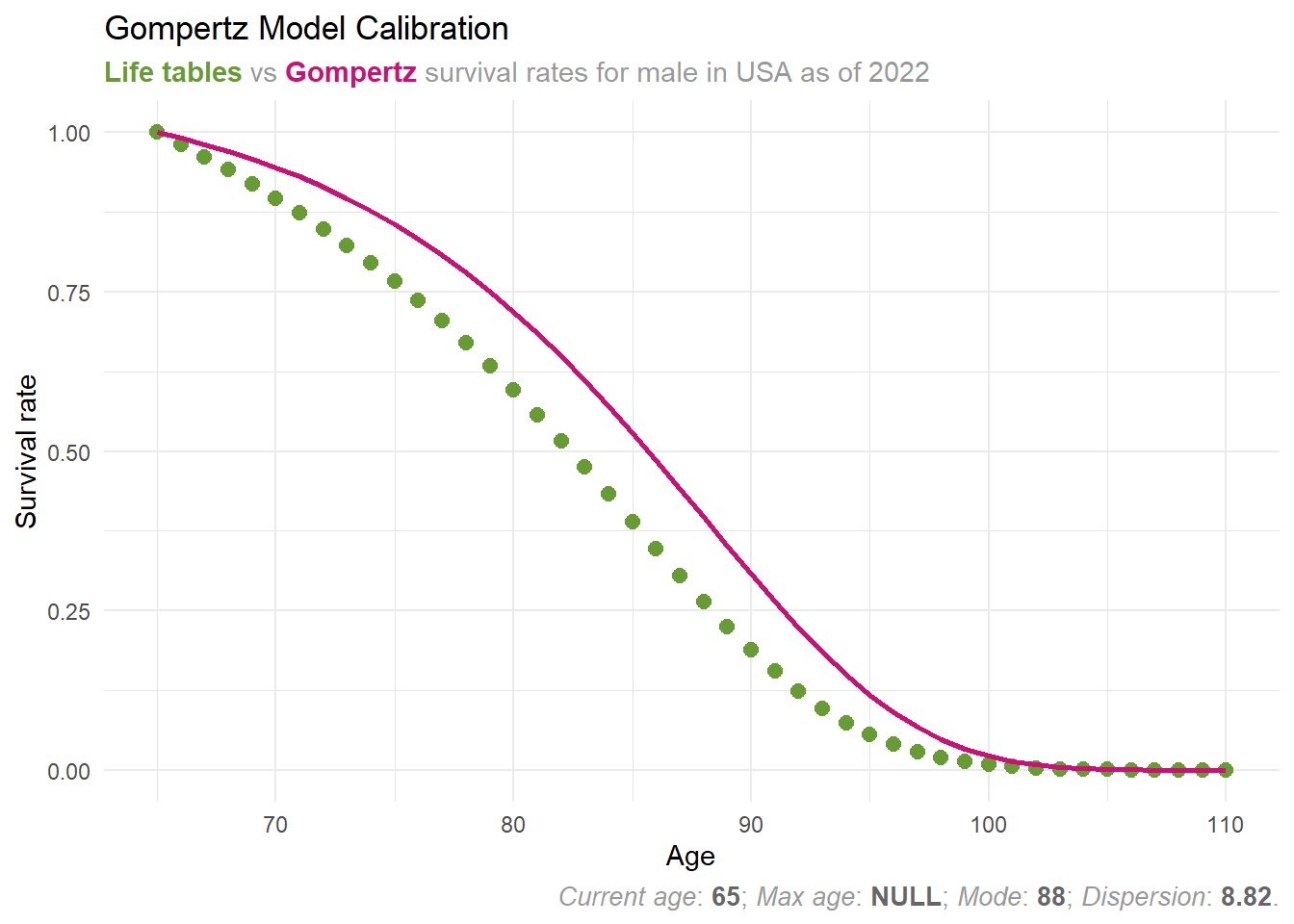
Thus, he wants to adjust the Gompertz parameters to be even more optimistic. One way to do this is by increasing the mode parameter. In this case we decide to add two years to the mode parameter to account for more optimistic survival probabilities.
Now that we have the Gompertz model parameters for both a female and a male, what happens if they are a couple and wish to combine their survival probabilities into a single Gompertz model?
Joint survival probabilities
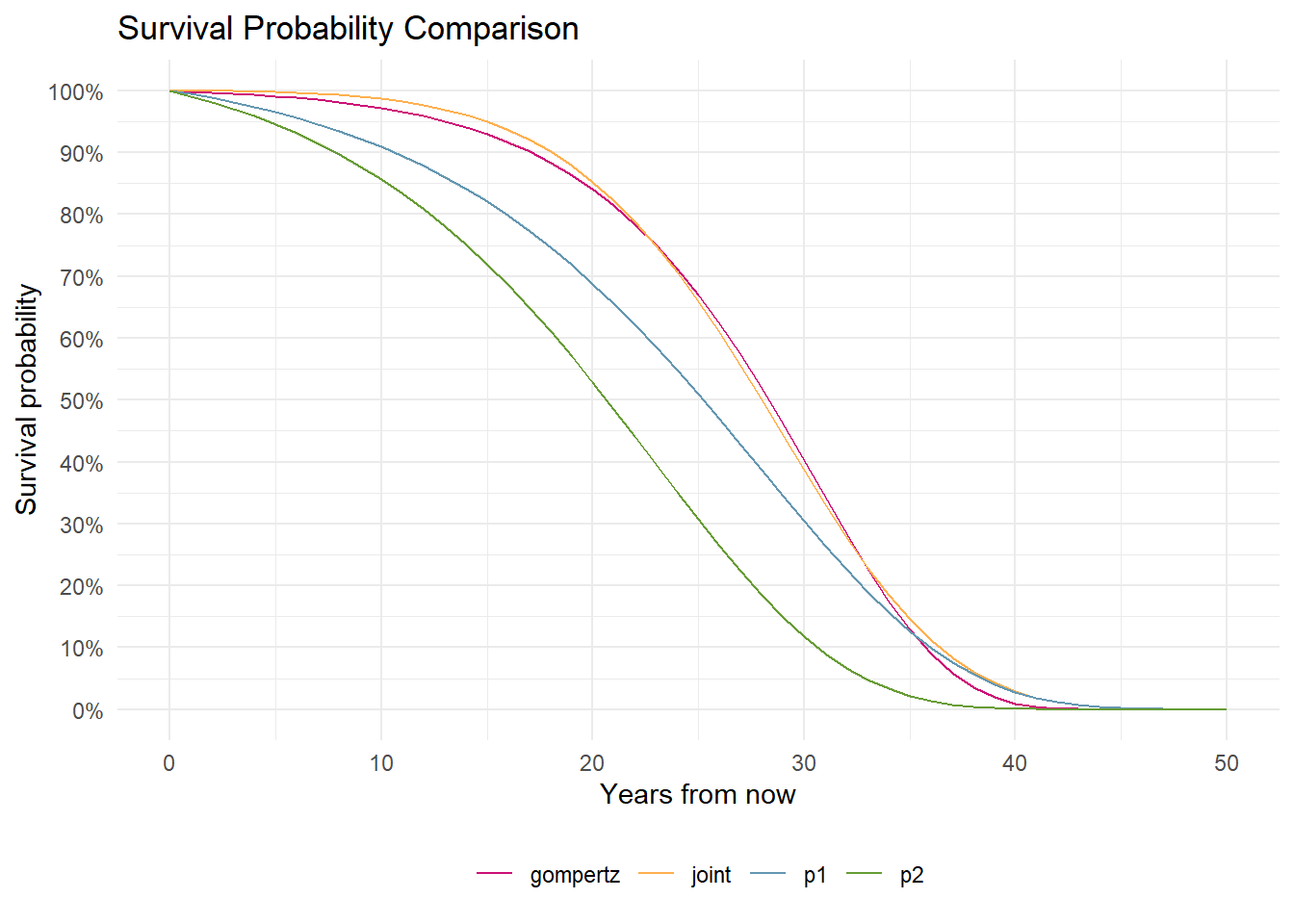
In a household with a couple, we might want to jointly model their survival probabilities to determine how long retirement might last when at least one member of the couple remains alive.
Our male subject, person 2 (p2), shows the lowest survival probabilities, while the female, person 1 (p1), has higher probabilities. However, their combined survival probabilities (of at least one surviving) are greater than the individual probabilities. Why does this matter? It’s important because as we will see in a moment considering only an individual will result in a lower retirement ruin probability than when considering a couple.
Calculating the retirement ruin probability
Now, we have gathered most of the information required to calculate the probability of retirement ruin. However, we still need the parameters for the distribution of yearly returns for our portfolio. Luckily for us, we have already discussed this topic in a previous post: How to Determine Our Optimal Asset Allocation?
When writing that post, we determined that the forward-looking mean of returns for the global stock market is approximately 4.49%. We assumed the standard deviation of returns to be around 15%.
Let’s use these inputs to determine the probability of retirement ruin for a 65-year-old male living in the USA. We assume more optimistic survival probabilities, with the Gompertz model parameter increased by 2.
Our male wants to retire at his current age (65 years) and start withdrawing from his portfolio. He plans to withdraw an inflation-adjusted $60,000 annually from his portfolio, which is currently valued at $1 million. This portfolio will be fully invested in an ETF tracking the global stock market.
The chance of outliving one’s retirement savings is nearly 25%. For a 65-year-old male, this suggests that in almost 25% of scenarios, he will run out of money during retirement. It’s not very comforting situation, is it?
Let’s compare retirement ruin probability of our 65-year-old male with a 60-year-old female (who also wants to retire at her current age). All other parameters are the same, except for those related to age and survival probabilities.
The probability of retirement ruin for a female is 1/3, which is higher than that for a 65-year-old man. This isn’t surprising because the woman in question is younger, and women typically have longer lifespans than men. Consequently, the funds must suffice for a more extended period during her retirement.
Comparing the ruin probabilities of individual versus joint retirement
What if we take into account the joint survival probabilities of the couple? We can use the age of the younger individual in the household as the starting point for the Gompertz model, in this case, the current age of the woman. We assume that they both want to retire at their current age, they plan to withdraw for the same household the same amount of money (60k) from the same portfolio (1m), just this time they consider themselves as a couple and taking into account each other survival probabilities.
As anticipated, the probability of retirement ruin for the couple is greater because the chance that at least one partner will still be alive is higher compared to an individual.
Now that we know how to calculate the probability of retirement ruin, let’s explore how this probability varies with different withdrawal rates.
What if we choose different withdrawal rates?
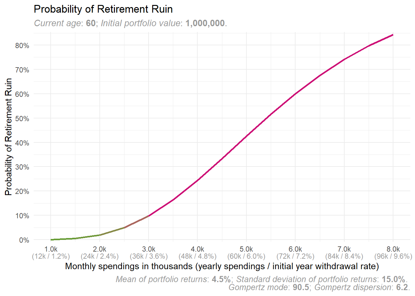
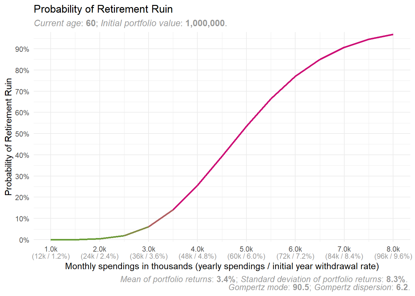
To analyse how various withdrawal rates affect the probability of retirement ruin for our previously defined couple, we can use the plot_retirement_ruin() function to generate a plot. We don’t need to specify monthly_spendings parameters, as the plot will automatically select default values for the spendings.
From the plot, you can observe that monthly spending below 3,000 results in a probability of ruin of less than 10%. A monthly spending of 3,000 (USD or any other currency) equates to 36,000 annually, representing 3.6% of the current portfolio value and our initial withdrawal rate.
Now we have everything necessary to examine some well-known assertions regarding Safe Withdrawal Rates (SWR). Let us begin with the most famous one: the 4% Rule.
4% Safe (or not?) Withdrawal Rate (SWR)
In Moshe Milevsky’s words: “If you haven’t heard of the infamous 4% rule of retirement income planning, it’s probably for the better. No single number has been more closely associated with retirement planning, and no single number has been so widely abused.” (Moshe A. Milevsky 2012)
The 4% Rule emerged in October 1994 when William Bengen published an article in the Journal of Financial Planning titled “Determining Withdrawal Rates Using Historical Data.” He suggested that starting with an initial 4% withdrawal in the first year, followed by inflation-adjusted withdrawals in subsequent years, should be safe based on historical data.
Many articles have been published about it since, but here, let’s focus on verifying this rule using our retirement ruin probability framework. Keeping all other assumptions constant, we’ll examine how a 4% withdrawal rate affects our retirement ruin probability.
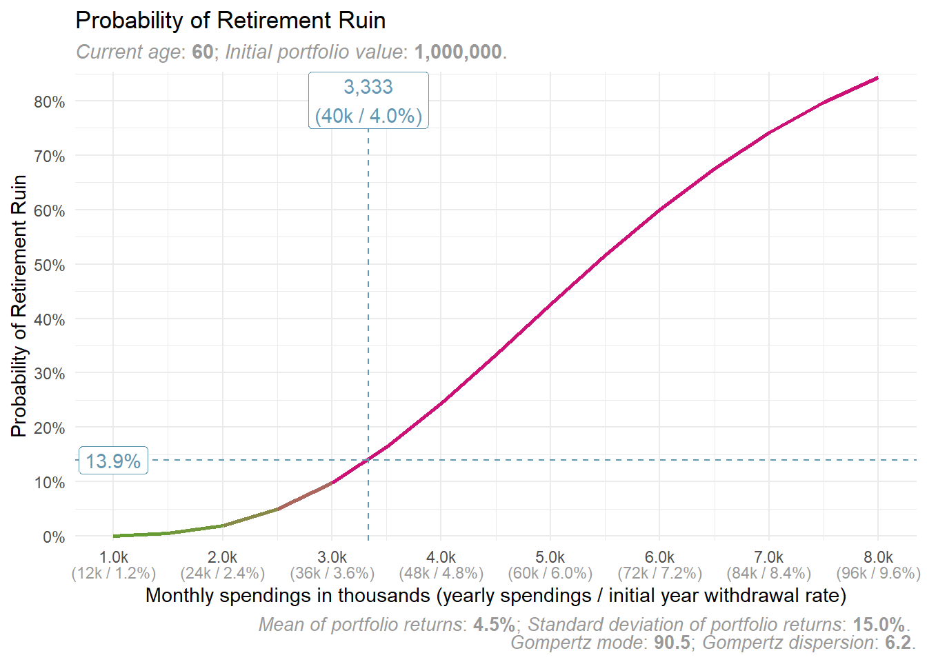
Let’s run the plot_retirement_ruin() function again for our couple, but this time set the monthly_spendings parameter to 4% of the portfolio value, then divide it by 12 to calculate the monthly spendings.
The plot indicates that with this withdrawal rate, there’s almost a 14% probability of retirement ruin. This isn’t insignificant. We will later discuss what an acceptable risk level might be.
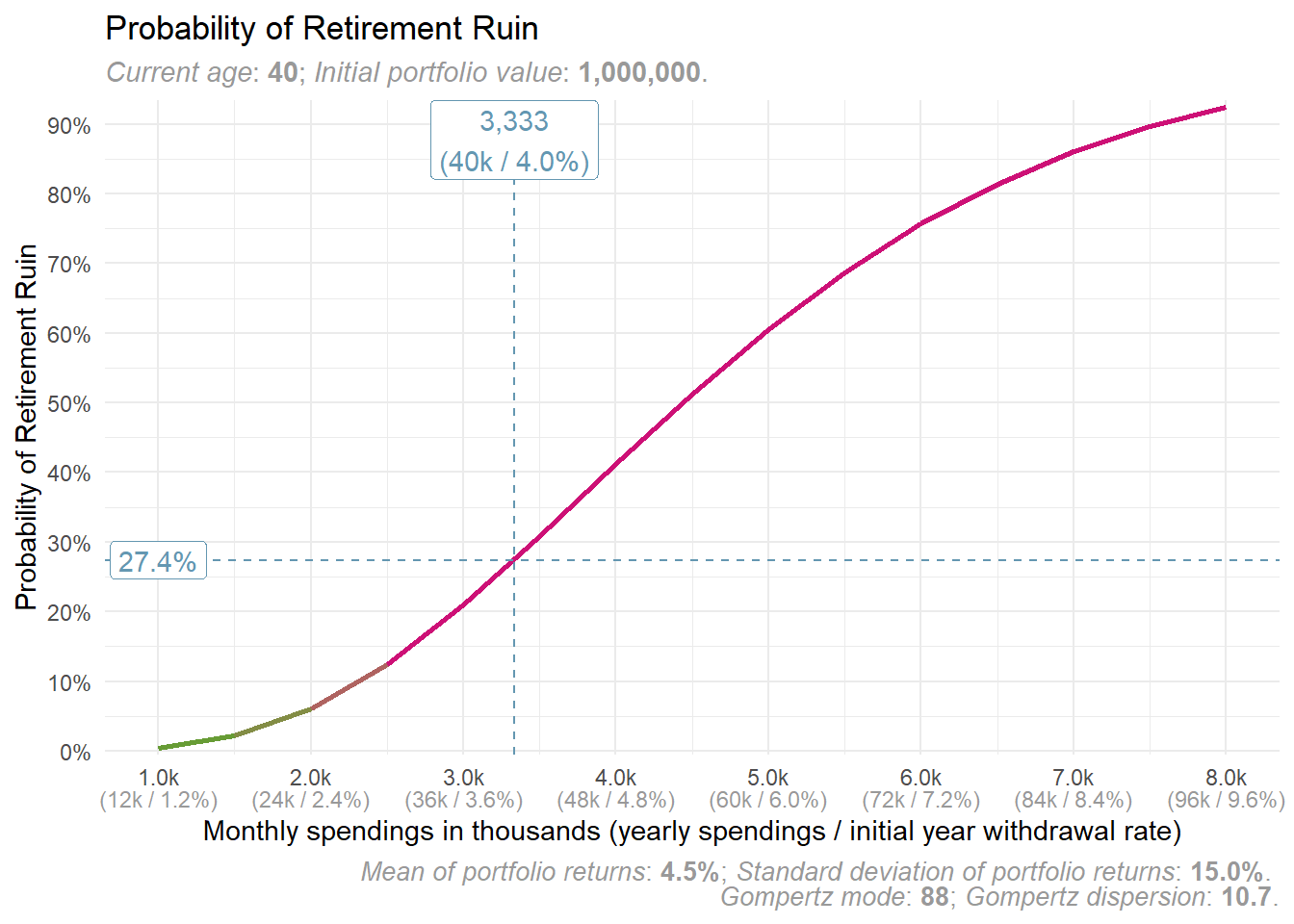
Now, let’s examine the 4% Rule for a single and younger person, specifically a 40-year-old female, who plans to retire at that age.
For a 40-year-old woman, the probability of financial ruin exceeds 27%. This suggests that the 4% Rule may not be reasonable for everyone, especially when considering the duration of retirement and potential changes in anticipated, forward-looking portfolio returns.
Some suggest that 8% is the new Safe Withdrawal Rate…(!?)
Occasionally, influencers introduce new claims about Safe Withdrawal Rates, like Dave Ramsey and 8% SWR. The issue is that personalities like Dave Ramsey hold significant influence and reach a vast audience, affecting their views. But what if their advice isn’t just suboptimal for many but also actually harmful?
In 2023, Dave Ramsey advised considering an 8% Safe Withdrawal Rate. However, this claim has been challenged in an article by David Blanchett, Michael Finke, and Wade Pfau titled “Supernerds Unite Against Dave Ramsey’s 8% Safe Withdrawal Rate Guidance” (D. Blanchett, Finke, and Pfau 2023) To add to the discussion, we will attempt to verify the 8% SWR using our retirement ruin probability framework.
Dave Ramsey’s logic is as follows: “If you’re making 12 [percent] in good mutual funds and the S&P is averaging 11.8, and if inflation for the last 80 years is 4%, if you make 12 and you need to leave 4% in there for average inflation raises, that leaves you eight. So, I’m perfectly comfortable drawing eight. But if you want to be a little bit conservative, seven. But, sure, not five or three. […] You put that out into the dadgum community and then people go ’I don’t have enough money. It’s hopeless. I’ll never be able to save enough to retire. A million dollars should be able to create an $80,000 income for you, boys and girls, perpetually! Forever! You should be able to pull $80,000 forever.” (D. Blanchett, Finke, and Pfau 2023)
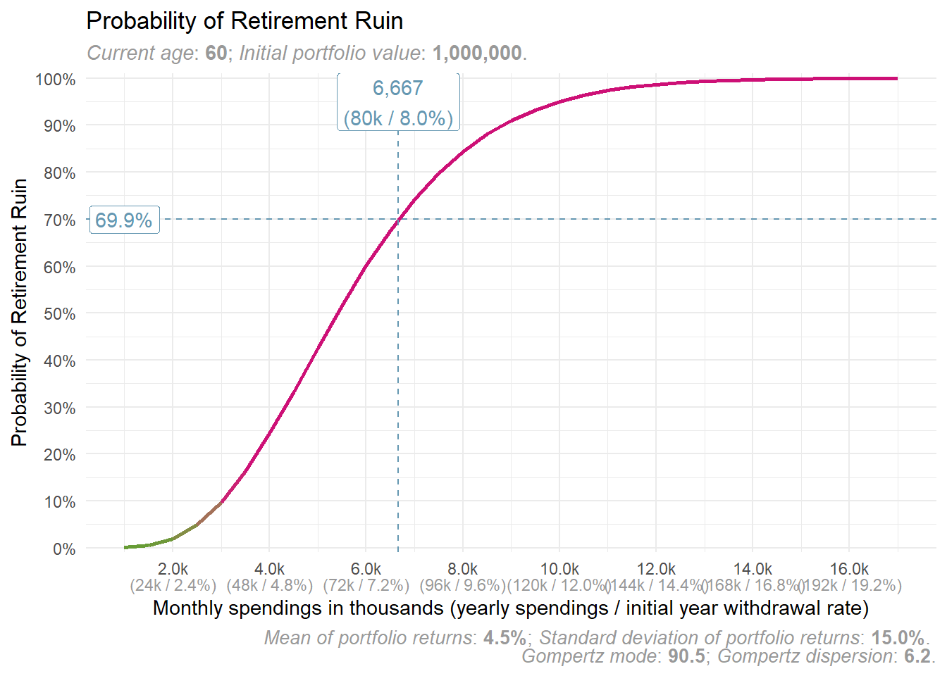
Following Ramsey’s advice, let’s see how the probability of ruin looks for our couple with 8% initial withdrawal rate.
The risk of ruin is nearly 70%! Would you consider taking such a risk and follow Ramsey’s advice? We would certainly not!
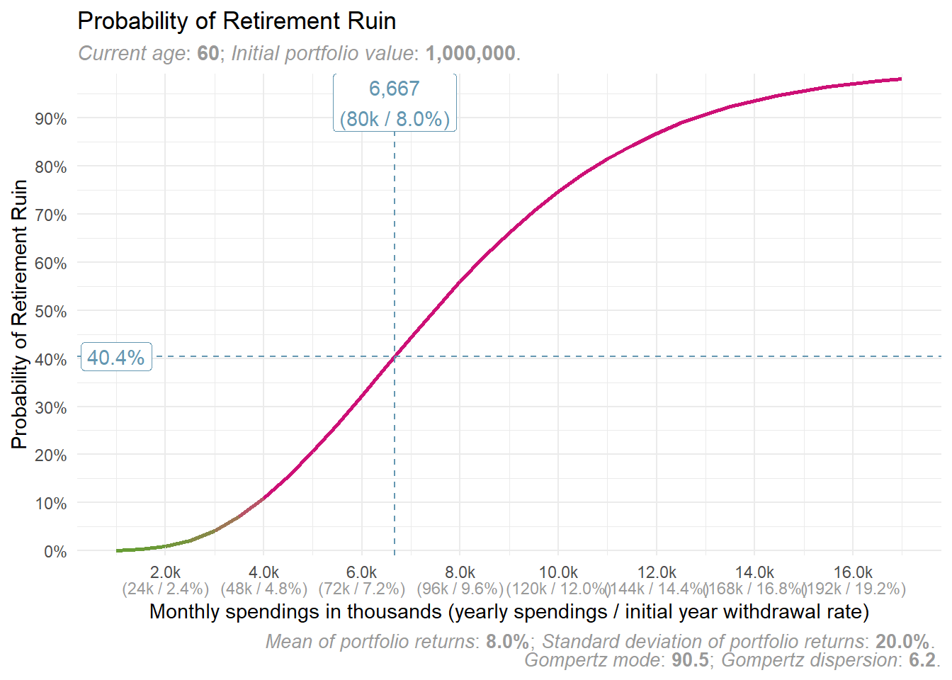
You might argue that we’re being unfair because Ramsey makes different assumptions regarding stock market returns. He believes the U.S. stock market will yield approximately 8% in real returns, above inflation. Let’s adjust this parameter in our function. Since we’re focusing solely on U.S. stocks, we must consider their higher volatility compared to the global market, which means adjusting the standard deviation as well.
While the probability of ruin is indeed lower, it still exceeds 40%. Even with these unrealistic long-term assumptions about stock market returns, it’s still a bad idea to follow Ramsey’s recommendation.
Again, the “Supernerds” captured this perfectly: “While Ramsey’s advice might be less depressing, it is also dangerous. […] no retiree should believe that they can maintain an $80,000 lifestyle after saving $1 million. They either need to save more, retire a little later, or spend less. Although reality is a little more depressing, it is still reality” (D. Blanchett, Finke, and Pfau 2023).
Now that we’ve covered changes in the withdrawal rate on the probability of retirement ruin, let’s take a look at the effect of portfolio diversification.
What is an effect of a portfolio diversification on retirement ruin probability?
The “Supernerds” also have something to say about diversifying portfolios: “No retiree should have their savings entirely in stocks. Bonds help buffer downturns, resulting in a higher safe withdrawal rate that comes from a lower sequence of return risk” (D. Blanchett, Finke, and Pfau 2023).
This aligns with M. Milevsky’s statements regarding the risk of retirement ruin: “Can you increase your sustainable spending rate without taking on additional risk? Believe it or not, the answer to this question is Yes. Let me explain. A retiree who invests “too much” money in risky equity funds will run the risk of retirement ruin if markets perform poorly during the first few years of retirement. On the other hand, investing “too little” in the equity fund runs the same risk of retirement ruin but this time because there is insufficient portfolio growth to sustain the spending rate. It seems that you are “damned if you do and damned if you don’t.”(Moshe A. Milevsky 2006, 202)
In our previous post, How to Determine Our Optimal Asset Allocation?, we discussed the importance of having a diversified portfolio and how to establish an optimal allocation of assets between risky and safe options.
Let’s apply the assumptions and calculations from the previous post to determine the final probability of retirement ruin for our couple (65-year-old male and 60-year-old female). Additionally, we’ll assume their portfolio allocation to the risky asset matches the optimal risky asset allocation.
We can now compute the mean and standard deviation of the entire portfolio’s returns using simplified calculations, assuming no correlation between risky and safe assets.
For our couple the probability of retirement ruin seems to be close to zero, below 40k of real spendings per year. If they decide to adapt their initial withdrawal rate to 8%, they will face a retirement ruin with probability as high as Mount Everest and join Jorge and others who miscalculated and run out of money.
How does asset allocation impact the probability of retirement ruin?
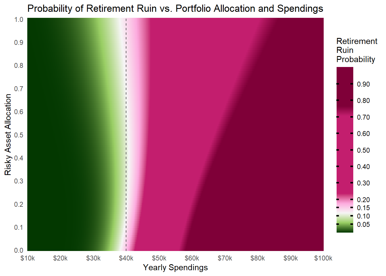
You might be curious about how the probability of retirement ruin changes with different portfolio allocations. The outcome largely depends on the initial withdrawal rate. Let’s explore what happens to the risk of retirement ruin when we adjust our portfolio allocation, particularly toward some extreme allocations.
Code
calc_portfolio_return_mean<-function(risky_asset_allocation, risky_asset_return_mean, safe_asset_return){(risky_asset_allocation*risky_asset_return_mean)+((1-risky_asset_allocation)*safe_asset_return)}calc_portfolio_return_sd<-function(risky_asset_allocation, risky_asset_return_sd){risky_asset_allocation*risky_asset_return_sd}grid_data<-tidyr::expand_grid( risky_asset_allocation =seq(0, 1, 0.01), yearly_spendings =seq(10000, 100000, 1000/5))|>dplyr::mutate( portfolio_return_mean =calc_portfolio_return_mean( risky_asset_allocation =risky_asset_allocation, risky_asset_return_mean =risky_asset_return_mean, safe_asset_return =safe_asset_return), portfolio_return_sd =calc_portfolio_return_sd( risky_asset_allocation =risky_asset_allocation, risky_asset_return_sd =risky_asset_return_sd), retirement_ruin =NA)for(iin1:nrow(grid_data)){grid_data[i, ]$retirement_ruin<-calc_retirement_ruin( portfolio_return_mean =grid_data$portfolio_return_mean[i], portfolio_return_sd =grid_data$portfolio_return_sd[i], age =min(params_female$current_age, params_male$current_age), gompertz_mode =params_joint$mode, gompertz_dispersion =params_joint$dispersion, portfolio_value =1000000, yearly_spendings =grid_data$yearly_spendings[i])}colours<-PrettyCols::prettycols("PinkGreens")grid_data|>ggplot2::ggplot(ggplot2::aes( x =yearly_spendings, y =risky_asset_allocation, fill =retirement_ruin))+ggplot2::geom_tile()+ggplot2::scale_fill_gradientn( breaks =c(seq(0, 0.2, by =0.05), seq(0.3, 1, by =0.1)), guide =ggplot2::guide_colorbar( barwidth =1.5, barheight =15, title.position ="top", ticks.colour ="black", ticks.linewidth =1), colours =c(colours[9],colours[6],rep(colours[5], 1),colours[4],rep(colours[2], 9),rep(colours[1], 5)), name ="Retirement\nRuin\nProbability")+ggplot2::geom_vline( xintercept =40000, linetype ="dashed", color ="gray30")+ggplot2::theme_minimal()+ggplot2::labs( title ="Probability of Retirement Ruin vs. Portfolio Allocation and Spendings", x ="Yearly Spendings", y ="Risky Asset Allocation")+ggplot2::scale_y_continuous( breaks =seq(0, 1, 0.1), expand =c(0, 0))+ggplot2::scale_x_continuous( breaks =seq(10000, 100000, 10000), expand =c(0, 0), labels =scales::dollar_format( scale =1e-3, suffix ="k"))
For high annual withdrawals (in this case exceeding $40,000), a portfolio heavily weighted towards safe assets increases the risk of depleting retirement funds (indicated in dark red). This makes sense since these portfolios lack growth potential. The only way funds might last is if you have a shorter lifespan, which isn’t a risk to depend on. However, with higher withdrawals, the risk of running out of money is unacceptable, regardless of how much is allocated to risky assets.
If the withdrawals remain reasonably low (indicated in green, with darker shades being better), the chance of ruin is relatively low. Allocating either too much or too little to risky assets increases the probability of ruin compared to building a more balanced portfolio.
Naturally, the less we withdraw, the lower the probability of ruin (indicated by darker green), but this doesn’t imply we should deny ourselves in retirement. Instead, we should aim to find an optimal balance between withdrawals and returns of our portfolio to sustain our reasonable standard of living.
We will explore this topic further in upcoming posts. But as of now, is it advisable to rely (only) on retirement ruin probability for planning your retirement? We believe it is not.
Why is the probability of retirement ruin likely not the optimal tool for retirement planning?
The metrics have several issues:
The probability of retirement ruin indicates the chance that you might deplete your funds during retirement. However, it doesn’t specify when you’ll run out of money —early into retirement or maybe just before reaching your maximum possible age.
Living to an advanced age is much less likely than surviving to next year. Therefore, it might make sense to plan for smaller incomes in the distant future if the chance of being alive to enjoy those incomes is low.(Sharpe 2019, 554) Or even that it could be optimal to “exhaust your investment portfolio and live off pension income by some advanced age. If so, ruin shouldn’t be feared.”(Moshe A. Milevsky 2016, 9)
The concept of retirement ruin suggests maintaining a constant spending rate in real dollars annually, regardless of the portfolio’s performance. But what if the portfolio performance is poor? Should we continue spending the same real amount each year?
The smaller the chance of “running out of money,” the greater the likelihood that a substantial amount of money will be left unspent, then provided to an estate (Sharpe 2019, 555). What if we don’t intend to leave large estate? Or what if we prefer to set aside a specific amount, but use the rest during our lifetime, so we can witness the positive impact our money can have on others?
What happens if our spending strategy or financial needs evolve over time? Following a fixed spending schedule isn’t practical. People adjust to new financial conditions, and no one (usually) waits until they’re entirely ruined to begin fixing their finances.(Moshe Arye Milevsky 2020, 176).
As William Sharpe put it succinctly: “[…] putting the subject in non-academic terms: it just seems silly to finance a constant, non-volatile spending plan using a risky, volatile investment strategy.” (Sharpe 2019, 513)
Finally, as M. Milevsky pointed out, the “problem with probabilities as guiding risk metric - nobody agrees on how much shortfall probability is acceptable in the context of retirement income planning. Is 10% too high? […] would you get on an airplane with a 0.1% probability of failure? Why should a retirement plan be any different? Do you see the problem?”(Moshe A. Milevsky 2016, 8). One might argue that minimizing the risk of ruin is essential. However, taken to the extreme, this could result in indefinitely postponing retirement or unnecessarily lowering our standard of living. We certainly want to avoid these outcomes.
This metric on its own is not the ideal tool for planning our retirement, but for what purpose might it be sufficient?
For what purpose is the retirement ruin probability a useful tool?
We agree that we shouldn’t rely too heavily on the probability of retirement ruin. However, it can be useful for a quick sanity check. This allows us to swiftly evaluate either our own or someone else’s assumptions about constant withdrawal rates in specific economic conditions, while also considering individual survival probabilities.
How should we interpret this metric?
If the probability of ruin isn’t close to zero, you should reconsider your decisions carefully. How close to zero is considered “good enough”? That’s a subjective threshold and hard to define. However, it’s certain that a 40% probability isn’t deemed “good enough.”
Perhaps it’s sufficient for Ramsey, but it isn’t for us, Jorge (he found out the hard way), or likely for you. Would you gamble your retirement on a single coin toss? We wouldn’t. We only get one chance at life and retirement, and we don’t want to waste it.
Topics to study further
We believe that while some decisions are better than others, optimal decisions are the best.
We aim to focus on how to achieve these optimal decisions, and for that reason, we need to use more advanced tools than Save Withdrawal Rates, constant spending strategies, and the probability of retirement ruin.
An alternative to constant spending is dynamic spending based on life-cycle model. This method links spending to portfolio performance, taking into account factors like survival probabilities, net worth, liabilities, and essential expenses. In our upcoming posts, we intend to discuss these approaches for making optimal financial decisions.
Try our interactive web apps
Tip
You can use your own customized inputs with our interactive web apps, that can be found on the Tools page.
Blanchett, David M., and Paul D. Kaplan. 2013. “Alpha, Beta, and Now... Gamma.”The Journal of Retirement 1 (2): 29–45. https://doi.org/10.3905/jor.2013.1.2.029.
Human Mortality Database. 2025. “Human Mortality Database.” Max Planck Institute for Demographic Research (Germany), University of California, Berkeley (USA),; French Institute for Demographic Studies (France); https://www.mortality.org.
Idzorek, Thomas M., and Paul D. Kaplan. 2024. Lifetime Financial Advice: A Personalized Optimal Multilevel Approach. CFA Institute Research Foundation.
Milevsky, Moshe A. 2006. The Calculus of Retirement Income: Financial Models for Pension Annuities and Life Insurance. Cambridge University Press.
Milevsky, Moshe A., and Chris Robinson. 2005. “A Sustainable Spending Rate Without Simulation.”Financial Analysts Journal 61 (6): 89–100. https://doi.org/10.2469/faj.v61.n6.2776.
Milevsky, Moshe Arye, and Chris Robinson. 2000. “Self-Annuitization and Ruin in Retirement.”North American Actuarial Journal 4 (4): 112–24. https://doi.org/10.1080/10920277.2000.10595940.
Roser, Max. 2018. “Twice as Long – Life Expectancy Around the World.”Our World in Data.
———. 2020. “The Rise of Maximum Life Expectancy.”Our World in Data.
DISCLAIMER! The content on this blog is provided solely for educational purposes. It does not constitute any form of investment advice, recommendation to buy or sell any securities, or suggestion to adopt any investment strategy. Any investment strategies and results discussed herein are for illustration purposes only.
The content reflects the observations and views of the author(s) at the time of writing, which are subject to change at any time without prior notice. The information is derived from sources deemed reliable by the authors, but its accuracy and completeness cannot be guaranteed. This material does not take into account specific investment objectives, financial situations, or the particular needs of any individual reader. Any views regarding future outcomes may or may not materialize. Past performance is not indicative of future results.
This content is not investment advice or information recommending or suggesting an investment strategy within the meaning of Article 20(1) of Regulation (EU) No 596/2014 of the European Parliament and of the Council of 16 April 2014 on market abuse.
Investing always involves risks, and any investment decisions are made at your own responsibility.